TrategyMulti-Indicator Trading System - Detailed Description
═══════════════════════════════════════════
OVERVIEW
This indicator combines four proven technical analysis tools (EMA, RSI, MACD, ATR) with a specific logic that filters out low-probability setups. Unlike simple indicator mashups, this system requires all conditions to align simultaneously before generating a signal, significantly reducing false entries.
═══════════════════════════════════════════
CORE COMPONENTS & LOGIC
1. Trend Detection - Triple EMA Filter
The system uses three Exponential Moving Averages (5, 10, 20 periods) to establish trend direction and strength:
For LONG signals:
• EMA(5) must be above EMA(10)
• EMA(10) must be above EMA(20)
• Price must be trading above all three EMAs
This creates a "stacked EMA" configuration that confirms a strong uptrend.
For SHORT signals:
• EMA(5) must be below EMA(10)
• EMA(10) must be below EMA(20)
• Price must be trading below all three EMAs
This inverse configuration confirms a strong downtrend.
2. Momentum Confirmation - RSI Filter
The RSI (14-period) acts as a momentum filter to avoid entering during exhausted moves:
For LONG signals:
• RSI must be above 40 (avoiding oversold extremes)
• RSI must be rising (current RSI > previous RSI)
For SHORT signals:
• RSI must be below 60 (avoiding overbought extremes)
• RSI must be falling (current RSI < previous RSI)
This prevents entries at extreme overbought/oversold levels while confirming momentum direction.
3. Entry Trigger - MACD Crossover
The MACD (12, 26, 9) provides the precise entry timing:
LONG trigger: MACD line crosses above Signal line
SHORT trigger: MACD line crosses below Signal line
The signal only fires when this crossover occurs while all other conditions are already met.
4. Risk Management - ATR-Based TP/SL
Take Profit and Stop Loss levels are calculated dynamically using the 14-period ATR (Average True Range), adjusted for timeframe:
5-Minute Charts:
• Take Profit: 1.0 × ATR
• Stop Loss: 0.5 × ATR
4-Hour Charts and above:
• Take Profit: 2.0 × ATR
• Stop Loss: 1.0 × ATR
This adaptive approach accounts for different volatility levels across timeframes.
═══════════════════════════════════════════
SIGNAL GENERATION LOGIC
A signal is only generated when ALL four conditions are simultaneously true:
LONG Signal Requirements:
1. ✓ Triple EMA alignment (bullish stack)
2. ✓ Price above all EMAs
3. ✓ RSI > 40 and rising
4. ✓ MACD bullish crossover
SHORT Signal Requirements:
1. ✓ Triple EMA alignment (bearish stack)
2. ✓ Price below all EMAs
3. ✓ RSI < 60 and falling
4. ✓ MACD bearish crossover
This multi-layered filtering approach is what differentiates this system from basic indicator combinations.
═══════════════════════════════════════════
WHY THIS COMBINATION WORKS
Trend + Momentum + Timing:
• EMAs establish the overall trend context
• RSI confirms momentum is present (not exhausted)
• MACD provides precise entry timing
• ATR adapts risk management to current volatility
Key Innovation: The system waits for all filters to align rather than acting on individual signals, which significantly reduces whipsaws and false breakouts common in single-indicator strategies.
═══════════════════════════════════════════
OPTIMIZED TIMEFRAMES
While the indicator works on all timeframes, it has been specifically optimized and backtested on:
• 5-minute charts (for scalping/day trading)
• 4-hour charts (for swing trading)
The ATR multipliers automatically adjust based on the selected timeframe.
═══════════════════════════════════════════
VISUAL FEATURES
• Green arrows below bars: Long signal
• Red arrows above bars: Short signal
• Green line: Take Profit level
• Red line: Stop Loss level
• Alert capability: Configurable alerts for paid TradingView subscriptions
═══════════════════════════════════════════
HOW TO USE
1. Add the indicator to your chart
2. Wait for a colored arrow to appear
3. Enter the trade in the direction of the arrow
4. Set your Take Profit at the green line
5. Set your Stop Loss at the red line
6. (Optional) Set up alerts to receive notifications
Note: Not every arrow will show TP/SL lines. Lines only appear when the ATR-based calculation determines there is sufficient volatility to justify the trade setup.
═══════════════════════════════════════════
WHAT MAKES THIS INVITE-ONLY WORTHY
Unlike free indicators that simply plot standard EMAs, RSI, or MACD separately, this system:
1. Integrates all four indicators with specific thresholds designed to work together
2. Uses adaptive risk management that adjusts to timeframe and volatility
The value lies not in the individual components (which are public domain) but in the specific combination logic, thresholds, and ATR-based risk system that took months of testing to optimize.
═══════════════════════════════════════════
ACCESS INFORMATION
This is an invite-only indicator. To request access:
• Visit our website
We offer both monthly subscriptions and lifetime access.
═══════════════════════════════════════════
RISK DISCLAIMER
This indicator is a technical analysis tool and does not constitute financial advice. All trading involves substantial risk of loss. Past performance does not guarantee future results. The indicator provides signals based on historical price patterns, but cannot predict future market movements. Always use proper risk management and never risk more than you can afford to lose.
═══════════════════════════════════════════
Questions? Feel free to message us on TradingView, or to email us.
Cari dalam skrip untuk "swing trading"

Key Support and ResistanceKEY SUPPORT AND RESISTANCE - USER GUIDE
========================================
OVERVIEW
This indicator automatically identifies and displays key support and resistance levels based on swing highs and swing lows. It uses pivot point detection to mark significant price levels where the market has previously shown reactions, helping traders identify potential entry/exit points and key decision zones.
KEY FEATURES
• Automatic Level Detection: Identifies swing highs (resistance) and swing lows (support) using pivot point analysis
• Dynamic Line Management: Displays only recent levels within a specified lookback period to keep charts clean
• Auto-Extending Lines: Projects support/resistance levels forward to anticipate future price interactions
• Color-Coded Levels: Red lines for resistance, green lines for support for easy visual identification
========================================
PARAMETERS
========================================
Left Bars (Default: 10)
• Minimum: 5 bars
• Number of bars to the left of the pivot point
• Higher values = more significant levels but fewer signals
• Lower values = more sensitive detection but may include minor swings
Right Bars (Default: 10)
• Minimum: 5 bars
• Number of bars to the right of the pivot point
• Must be confirmed by price action before the level is drawn
• Balances between confirmation delay and signal accuracy
Show Last N Bars (Default: 200)
• Minimum: 10 bars
• Only displays support/resistance levels detected within the most recent N bars
• Keeps your chart clean by removing outdated levels
• Adjust based on your trading timeframe and style
Line Extension Length (Default: 48)
• Minimum: 1 bar
• How many bars forward the support/resistance lines extend
• Helps visualize potential future price interactions
• Longer extensions useful for swing trading, shorter for day trading
========================================
HOW TO USE
========================================
FOR SWING TRADERS
1. Use default settings (10/10) or increase to 15/15 for more significant levels
2. Set "Show Last N Bars" to 300-500 to capture longer-term levels
3. Look for price reactions when approaching these levels
4. Combine with volume analysis for confirmation
FOR DAY TRADERS
1. Consider reducing Left/Right Bars to 7-8 for more frequent signals
2. Set "Show Last N Bars" to 100-150 to focus on recent action
3. Reduce "Line Extension Length" to 20-30 bars
4. Watch for intraday bounces or breakouts at these levels
TRADING STRATEGIES
Bounce Trading (Mean Reversion)
• Enter long when price approaches green support lines
• Enter short when price approaches red resistance lines
• Use stop loss just beyond the support/resistance level
• Best in ranging or consolidating markets
Breakout Trading (Trend Following)
• Wait for price to break through resistance (bullish) or support (bearish)
• Confirm with increased volume
• Previous resistance becomes new support (and vice versa)
• Best in trending markets
Multi-Timeframe Analysis
• Check higher timeframe levels for major support/resistance zones
• Use lower timeframe levels for precise entry/exit timing
• Confluence of multiple timeframe levels creates strong zones
========================================
IMPORTANT NOTES
========================================
Line Confirmation Delay
• Lines appear with a delay equal to "Right Bars" parameter
• This delay ensures the pivot point is confirmed
• Real-time level detection requires price action confirmation
Chart Clarity
• Maximum 500 lines can be displayed (TradingView limitation)
• Adjust "Show Last N Bars" if chart becomes too cluttered
• Old lines automatically delete when outside the lookback period
False Signals
• Not all support/resistance levels will hold
• Use additional confirmation (volume, candlestick patterns, other indicators)
• Markets can break through levels, especially during high-impact news
BEST PRACTICES
1. Combine with Other Analysis: Use alongside trend indicators, volume, and price action patterns
2. Context Matters: Consider overall market trend and structure
3. Risk Management: Always use stop losses; don't rely solely on S/R levels
4. Market Conditions: More effective in liquid, actively traded markets
5. Backtesting: Test settings on your specific instrument and timeframe before live trading
TROUBLESHOOTING
Too Many Lines?
• Increase "Left Bars" and "Right Bars" values
• Decrease "Show Last N Bars" value
Too Few Lines?
• Decrease "Left Bars" and "Right Bars" values
• Increase "Show Last N Bars" value
Lines Not Appearing?
• Ensure sufficient price data is loaded on your chart
• Check that "Right Bars" have passed since the last swing point
• Verify indicator is properly loaded (refresh if needed)
TECHNICAL DETAILS
• Uses ta.pivothigh() and ta.pivotlow() functions for level detection
• Implements array-based line management for efficient rendering
• Automatic cleanup of outdated lines to maintain performance
• Overlay indicator - displays directly on price chart
Disclaimer: This indicator is for educational and informational purposes only. It does not constitute financial advice. Always conduct your own research and risk assessment before making trading decisions.
========================================
中文使用指南
========================================
概述
本指標自動識別並顯示基於波段高點和低點的關鍵支撐阻力位。使用樞軸點檢測標記市場先前反應的重要價格水平,幫助交易者識別潛在的進出場點和關鍵決策區域。
主要功能
• 自動水平檢測:使用樞軸點分析識別波段高點(阻力)和波段低點(支撐)
• 動態線條管理:僅顯示指定回看期內的近期水平,保持圖表清晰
• 自動延伸線條:將支撐阻力水平向前投影,預測未來價格互動
• 顏色編碼:紅線表示阻力,綠線表示支撐,便於視覺識別
========================================
參數說明
========================================
左側K棒數(預設:10)
• 最小值:5根K棒
• 樞軸點左側的K棒數量
• 數值越高 = 水平越重要但訊號越少
• 數值越低 = 檢測更敏感但可能包含次要波動
右側K棒數(預設:10)
• 最小值:5根K棒
• 樞軸點右側的K棒數量
• 必須經過價格行為確認後才繪製水平
• 在確認延遲和訊號準確性之間取得平衡
顯示最近N根K棒內的點(預設:200)
• 最小值:10根K棒
• 僅顯示最近N根K棒內檢測到的支撐阻力水平
• 透過移除過時水平保持圖表清晰
• 根據您的交易時間框架和風格調整
線條延伸長度(預設:48)
• 最小值:1根K棒
• 支撐阻力線向前延伸的K棒數
• 幫助視覺化潛在的未來價格互動
• 較長延伸適合波段交易,較短適合當沖交易
========================================
使用方法
========================================
波段交易者
1. 使用預設設定(10/10)或增加至15/15以獲得更重要的水平
2. 將「顯示最近N根K棒」設為300-500以捕捉長期水平
3. 觀察價格接近這些水平時的反應
4. 結合成交量分析進行確認
當沖交易者
1. 考慮將左右側K棒減少至7-8以獲得更頻繁的訊號
2. 將「顯示最近N根K棒」設為100-150以專注於近期行情
3. 將「線條延伸長度」減少至20-30根K棒
4. 觀察日內在這些水平的反彈或突破
交易策略
反彈交易(均值回歸)
• 當價格接近綠色支撐線時做多
• 當價格接近紅色阻力線時做空
• 在支撐阻力水平之外設置止損
• 在區間或盤整市場中效果最佳
突破交易(趨勢跟隨)
• 等待價格突破阻力(看漲)或支撐(看跌)
• 以增加的成交量確認
• 先前的阻力成為新的支撐(反之亦然)
• 在趨勢市場中效果最佳
多時間框架分析
• 檢查更高時間框架的主要支撐阻力區域
• 使用較低時間框架進行精確的進出場時機
• 多個時間框架水平的匯合創造強大區域
========================================
重要注意事項
========================================
線條確認延遲
• 線條出現時會有等於「右側K棒數」參數的延遲
• 此延遲確保樞軸點被確認
• 實時水平檢測需要價格行為確認
圖表清晰度
• 最多可顯示500條線(TradingView限制)
• 如果圖表變得太雜亂,請調整「顯示最近N根K棒」
• 超出回看期的舊線會自動刪除
假訊號
• 並非所有支撐阻力水平都會守住
• 使用額外確認(成交量、K棒型態、其他指標)
• 市場可能突破水平,特別是在重大新聞期間
最佳實踐
1. 結合其他分析:與趨勢指標、成交量和價格行為型態一起使用
2. 背景很重要:考慮整體市場趨勢和結構
3. 風險管理:始終使用止損;不要僅依賴支撐阻力水平
4. 市場條件:在流動性高、活躍交易的市場中更有效
5. 回測:在實盤交易前,在您的特定商品和時間框架上測試設定
故障排除
線條太多?
• 增加「左側K棒數」和「右側K棒數」數值
• 減少「顯示最近N根K棒」數值
線條太少?
• 減少「左側K棒數」和「右側K棒數」數值
• 增加「顯示最近N根K棒」數值
線條未出現?
• 確保圖表上載入了足夠的價格數據
• 檢查自上次波動點以來是否已過「右側K棒數」
• 驗證指標是否正確載入(如需要請刷新)
技術細節
• 使用 ta.pivothigh() 和 ta.pivotlow() 函數進行水平檢測
• 實施基於陣列的線條管理以實現高效渲染
• 自動清理過時線條以保持性能
• 疊加指標 - 直接顯示在價格圖表上
免責聲明:本指標僅供教育和資訊目的。不構成財務建議。在做出交易決策前,請務必進行自己的研究和風險評估。

Simulated Liquidation Heatmap [QuantAlgo]🟢 Overview
This indicator visualizes where clusters of stop-loss orders and liquidation levels are likely located, displayed as a 'heatmap'. It's based on the concept of market structure liquidity: large groups of stop orders tend to gather around obvious technical levels (like swing highs and lows), and these pools of orders often attract price movement from institutional traders. The indicator uses a fractal-based algorithm to identify these high-probability liquidation zones and displays them as dynamic, color-coded boxes.
The key feature is the thermal color gradient, which indicates the freshness (age) and therefore the relative relevance of the liquidity zone. Hot colors (e.g., Red/Yellow) represent fresh clusters that have just formed, suggesting strong and immediate liquidity interest. Cold colors (e.g., Blue/Purple) represent aged or decaying clusters that are becoming less relevant over time. This visualization allows traders to anticipate potential liquidity sweeps (stop hunts) and understand areas of significant retail and institutional positioning.
🟢 Key Features
1. Liquidity Zone Heatmap
The core function is the identification of swing high and swing low price points using a user-defined Lookback period. These points are where retail traders are statistically most likely to place their stop-loss orders. The indicator simulates the clustering of these orders by drawing a zone (box) around the detected swing point, with the vertical size controlled by the Stop/Liquidation Zone Width (%) setting.
▶ Cluster Lookback: Defines the sensitivity of swing point detection. Lower values detect frequent, minor zones (scalping/intraday); higher values detect major, stronger swing points (swing trading).
▶ Zone Width (%): Sets the percentage range above and below the swing point where stops are simulated to cluster, accounting for slippage and typical stop placement spread.
▶ Liquidity Decay: Zones gradually fade in color intensity and are eventually removed after the user-defined Liquidity Decay Period (Bars), ensuring the heatmap only displays relevant, current liquidity areas.
▶ Round Number Filter: An optional filter that limits the display to liquidity zones occurring only at psychologically significant round numbers (e.g., $100, $1,500.00), which typically attract higher concentrations of orders.
2. Thermal Color Gradient
The heatmap's color is a direct function of the zone's age, providing a visual proxy for immediate relevance.
▶ Freshness: Newly created zones are displayed in the Hot Color (high relevance).
▶ Decay: As bars pass, the zone color transitions along the gradient toward the Cold Color and increased transparency (lower relevance), until it is removed entirely.
▶ Color Schemes: Multiple pre-configured and custom color schemes are available to optimize the visualization for different chart themes and color preferences.
3. Liquidity Heat Thermometer
An optional visual thermometer is displayed on the chart to provide an instant, overall assessment of the current liquidation heat level in the immediate vicinity of the price.
▶ Calculation: The thermometer calculates an aggregate heat score based on the age and proximity of all liquidity zones within a user-defined Zone Detection Range (%) of the current price.
▶ Visual Feedback: A marker (triangle) points to the corresponding level on the thermometer's color gradient (Hot to Cold). A high reading indicates price is close to fresh, dense stop clusters, suggesting high volatility or an imminent liquidity sweep is probable. A low reading indicates price is in a low-density or aged liquidity area.
▶ Customization: The thermometer's resolution, position, and text size are fully customizable for optimal chart placement and readability.
🟢 Practical Applications
▶ Anticipate Sweeps: Prioritize trading in the direction of Hot (fresh) liquidity zones. For example, a hot low-side zone suggests strong sell-side liquidity (stop-losses) is available for large buyers to sweep.
▶ Filter Noise: Use the Round Number Filter to focus only on the highest probability liquidation zones, which are often at clean, psychological price levels.
▶ Validate Entries: Combine the Heat Thermometer with price action analysis. A rising heat level indicates increasing proximity to a major stop cluster, signaling a potential turn or an aggressive market move to sweep those stops.
▶ Risk Management: Understand that price often acts dynamically around these zones. High heat levels imply high risk/reward setups; stops should be placed strategically beyond the defined Liquidation Zone Width.
▶ Multi-Timeframe Context: Higher timeframes (e.g., Daily, 4-Hour) often reveal more significant, major liquidity zones. Use this indicator on lower timeframes (e.g., 5-min, 15-min) for execution, but prioritize zones that align with higher-timeframe structures.

True Trend (StevenCharts)Overview
True Trend (StevenCharts) is a next-generation technical analysis tool designed to automate the most subjective part of trading: Drawing Trendlines.
Whether you are scalping, day trading, or swing trading, identifying valid support and resistance channels is critical. This indicator uses a proprietary multi-timeframe momentum engine to objectively identify market pivots and automatically draw precise, high-probability trendlines (rays) on your chart.
The "True Trend" Engine
At the heart of this indicator is a custom algorithmic model that evaluates market structure across multiple timeframes simultaneously.
No Guesswork: Instead of manually connecting wicks, the script waits for specific algorithmic momentum peaks and troughs to determine exactly where a trend begins and ends.
Dynamic Generation: When the internal trend logic detects maximum strength, the indicator tracks the highest or lowest points of the move. When momentum shifts, it locks in a trendline that projects forward, creating dynamic support and resistance levels.
Key Features
Automated Ray Creation: Automatically draws Red (Bearish) and Green (Bullish) rays based on confirmed momentum shifts.
Clean Chart Logic: The script includes intelligent "cleanup" logic. If price breaks a trendline and confirms the break with sustained momentum, the line is automatically removed to keep your chart clean and focused on relevant data only.
High Volume Confirmation: The logic accounts for volume spikes to validate line breaks.
"SHIFT" Logic (Adaptive vs. Static)
This script features a powerful setting called "Turn SHIFT On":
ON (Adaptive Mode): Uses advanced logic to "leapfrog" trendlines. As price makes new structural highs or lows, the trendline adjusts and locks onto the most recent valid pivot points. This is ideal for active traders following a developing trend.
OFF (Static Mode): Draws independent, static trendlines from every valid pivot. This is useful for seeing the history of market structure and identifying older levels that may still act as support/resistance.
How to Use
Support & Resistance: Use the automatically generated rays as dynamic S/R levels.
Bullish Trend: Price should respect the Green rays as support.
Bearish Trend: Price should respect the Red rays as resistance.
Breakout/Reversal: When a localized trendline is deleted or broken, it signals a potential shift in market structure.
Settings
Turn 'SHIFT' On: Toggles between adaptive (moving) lines and static lines.
Show Highest/Lowest Only: Keeps the chart clean by focusing on the most dominant outer trends.
Ray Colors: Customizable colors for Up and Down trends.

Ved Order BlocksOverview
Ved Order Blocks identifies critical supply and demand zones where significant buying and selling pressure exists.
The indicator automatically detects, validates, and displays high-probability support/resistance areas on your chart.
What Makes This Indicator Unique?
Micro-Level Detection System:
This indicator uses a high-period Relative Strenght Index to detect micro-level crossovers.
The high period length is specifically chosen to create a smooth line that filters out market noise completely.
This smooth calculation allows the indicator to catch precise Important levels that shorter periods would miss.
Smart Zone Filtering:
Unlike traditional order block indicators that show every single zone (creating chart clutter), Ved Order Blocks only displays overlapping zones.
When multiple order blocks stack on top of each other at the same price level, it indicates strong market interest.
Single, isolated zones are automatically hidden from your chart - you only see high-quality confluence areas where multiple zones converge.
Continuous Zone Tracking:
The indicator continuously tracks all order blocks in the background.
It monitors which zones are forming and where they overlap.
Only when zones overlap with each other does the indicator display them on your chart.
This ensures you're only seeing the most important levels where multiple orders are stacked.
Strength-Based Classification:
When order blocks form near the momentum centerline (around 50 level) AND near major moving average levels, the indicator marks them as "Strong Bullish OB" or "Strong Bearish OB" with special colored borders.
These points are particularly powerful because they represent both momentum equilibrium and trend support/resistance - the good setup for significant market moves.
How It Works
Monitors Micro levels of Relative Strenght Index
Each level represents potential high-activity zones
This range filters out noise and captures only significant moves
Step 2: Zone Creation
When momentum crosses upward: Creates Bullish Order Block (demand zone)
When momentum crosses downward: Creates Bearish Order Block (supply zone)
Uses the candle's high and low at crossover point
Step 3: Confirmation Delay
New zones enter a "pending" queue
Must survive 6 bars (default) before appearing
This filters out false signals
Only validated zones show on chart
Step 4: Size Filter (Optional)
Removes zones larger than 1.5% of current price (default)
Large zones are often unreliable
Keeps only actionable zones
Step 5: Overlap Detection
Compares all active order blocks continuously
Tracks which zones are overlapping with each other
When 2+ zones overlap = Premium confluence zone
Overlapping zones get higher strength ratings
IMPORTANT: Only overlapping zones are displayed on chart
Single zones are tracked but not shown (reduces clutter)
This ensures you only see high-quality levels
Strong Orderblocks
Type 1: Centerline Zones (Yellow Border)
Order blocks that form when momentum is near the Centerline
Represents perfect balance between buyers and sellers
Often leads to explosive moves as equilibrium breaks
Type 2: Major MA Zones (Orange Border)
Order blocks that form near the major moving average
Represents alignment with long-term trend
Acts as major support/resistance for large market participants
Type 3: Super Strong Zones (Purple Border)
Order blocks that meet BOTH conditions simultaneously
Highest probability setups
Settings Explained
Core Settings
Bar Delay (Default: 6)
Bars to wait before showing zone
Higher = fewer but reliable zones
Lower = more zones but more false signals
Order Block Sensitivity (Default: 10)
Detection frequency adjustment
Range: 1-20
Show Last Order Blocks (Default: 500)
Maximum zones displayed
Prevents chart clutter
Mitigation Method
Close: Zone breaks when candle closes beyond it
Wick: Zone breaks when price wicks through it
Order Block Style
Candle Body: Uses only body (tighter zones)
Full Candle: Uses full candle with wicks
Filters
Use Volume for Strength (Default: ON)
Includes volume in strength calculation
Recommended to keep ON
Filter Out Large Order Blocks (Default: OFF)
Enable to remove oversized zones
Set max size as % of price (default 1.5%)
Show Only Strong Order Blocks (Default: OFF)
Only displays yellow/orange/purple zones
Hides standard white border zones
Strength Settings
Centerline Sensitivity (Default: 0.1)
Increase for more zones, decrease for fewer
Highlight Strong OBs (Default: ON)
Enables orange border feature
Proximity Threshold (Default: 0.2%)
0.2% = tight confluence
Increase for more highlights
Timeframe Settings
Scalping (1m-5m)
Bar Delay: 3-5
Show Last OBs: 100
Show Only Strong: ON
Mitigation: Wick
Day Trading (15m-1H)
Bar Delay: 6-8
Show Last OBs: 200
Show Only Strong: OFF
Mitigation: Close
Swing Trading (4H-Daily)
Bar Delay: 8-12
Show Last OBs: 300
Show Only Strong: ON
Mitigation: Close
Key Advantages:
Eliminates chart clutter by showing only overlapping zones
High-period calculation filters all market noise
Automatic strength classification with visual indicators
Works on all timeframes and markets
Fully customizable to match your trading style
Auto-removes broken zones to keep chart updated
Important Limitation:
This indicator uses long period calculations.
Due to these high period requirements, the indicator's performance may vary for free TradingView users who have limited historical data access.
This indicator is best suited for TradingView paid plan users (Essential, Plus, or Premium) as they have access to extensive historical data, which allows the indicator to calculate and display zones more accurately and consistently across all timeframes.

Linear Trajectory & Volume StructureThe Linear Trajectory & Volume Structure indicator is a comprehensive trend-following system designed to identify market direction, volatility-adjusted channels, and high-probability entry points. Unlike standard Moving Averages, this tool utilizes Linear Regression logic to calculate the "best fit" trajectory of price, encased within volatility bands (ATR) to filter out market noise.
It integrates three core analytical components into a single interface:
Trend Engine: A Linear Regression Curve to determine the mean trajectory.
Volume Verification: Filters signals to ensure price movement is backed by market participation.
Market Structure: Identifies previous high-volume supply and demand zones for support and resistance analysis.
2. Core Components and Logic
The Trajectory Engine
The backbone of the system is a Linear Regression calculation. This statistical method fits a straight line through recent price data points to determine the current slope and direction.
The Baseline: Represents the "fair value" or mean trajectory of the asset.
The Cloud: Calculated using Average True Range (ATR). It expands during high volatility and contracts during consolidation.
Trend Definition:
Bullish: Price breaks above the Upper Deviation Band.
Bearish: Price breaks below the Lower Deviation Band.
Neutral/Chop: Price remains inside the cloud.
Smart Volume Filter
The indicator includes a toggleable volume filter. When enabled, the script calculates a Simple Moving Average (SMA) of the volume.
High Volume: Current volume is greater than the Volume SMA.
Signal Validation: Reversal signals and structure zones are only generated if High Volume is present, reducing the likelihood of trading false breakouts on low liquidity.
Volume Structure (Smart Liquidity)
The script automatically plots Support (Demand) and Resistance (Supply) boxes based on pivot points.
Creation: A box is drawn only if a pivot high or low is formed with High Volume (if the volume filter is active).
Mitigation: The boxes extend to the right. If price breaks through a zone, the box turns gray to indicate the level has been breached.
3. Signal Guide
Trend Reversals (Buy/Sell Labels)
These are the primary signals indicating a potential change in the macro trend.
BUY Signal: Appears when price closes above the upper volatility band after previously being in a downtrend.
SELL Signal: Appears when price closes below the lower volatility band after previously being in an uptrend.
Pullbacks (Small Circles)
These are continuation signals, useful for adding to positions or entering an existing trend.
Long Pullback: The trend is Bullish, but price dips momentarily below the baseline (into the "discount" area) and closes back above it.
Short Pullback: The trend is Bearish, but price rallies momentarily above the baseline (into the "premium" area) and closes back below it.
4. Configuration and Settings
Trend Engine Settings
Trajectory Length: The lookback period for the Linear Regression. This is the most critical setting for tuning sensitivity.
Channel Multiplier: Controls the width of the cloud.
1.0: Aggressive. Results in narrower bands and earlier signals, but more false positives.
1.5: Balanced (Default).
2.0+: Conservative. Creates a wide channel, filtering out significant noise but delaying entry signals.
Signal Logic
Show Trend Reversals: Toggles the main Buy/Sell labels.
Show Pullbacks: Toggles the re-entry circle signals.
Smart Volume Filter: If checked, signals require above-average volume. Unchecking this yields more signals but removes the volume confirmation requirement.
Volume Structure
Show Smart Liquidity: Toggles the Support/Resistance boxes.
Structure Lookback: Defines how many bars constitute a pivot. Higher numbers identify only major market structures.
Max Active Zones: Limits the number of boxes on the chart to prevent clutter.
5. Timeframe Optimization Guide
To maximize the effectiveness of the Linear Trajectory, you must adjust the Trajectory Length input based on your trading style and timeframe.
Scalping (1-Minute to 5-Minute Charts)
Recommended Length: 20 to 30
Multiplier: 1.2 to 1.5
Logic: Fast-moving markets require a shorter lookback to react quickly to micro-trend changes.
Day Trading (15-Minute to 1-Hour Charts)
Recommended Length: 55 (Default)
Multiplier: 1.5
Logic: A balance between responsiveness and noise filtering. The default setting of 55 is standard for identifying intraday sessions.
Swing Trading (4-Hour to Daily Charts)
Recommended Length: 89 to 100
Multiplier: 1.8 to 2.0
Logic: Swing trading requires filtering out intraday noise. A longer length ensures you stay in the trade during minor retracements.
6. Dashboard (HUD) Interpretation
The Head-Up Display (HUD) provides a summary of the current market state without needing to analyze the chart visually.
Bias: Displays the current trend direction (BULLISH or BEARISH).
Momentum:
ACCELERATING: Price is moving away from the baseline (strong trend).
WEAKENING: Price is compressing toward the baseline (potential consolidation or reversal).
Volume: Indicates if the current candle's volume is HIGH or LOW relative to the average.
Disclaimer
*Trading cryptocurrencies, stocks, forex, and other financial instruments involves a high level of risk and may not be suitable for all investors. This indicator is a technical analysis tool provided for educational and informational purposes only. It does not constitute financial advice, investment recommendations, or a guarantee of profit. Past performance of any trading system or methodology is not necessarily indicative of future results.

HVN Smart Liquidity📊 What the Indicator Does
HVN Smart Liquidity is a professional tool for identifying institutional liquidity zones based on Market Profile analysis and High Volume Nodes (HVN). The indicator visualizes dynamic zones where the greatest trading activity is concentrated, using TPO (Time Price Opportunity) methodology to reveal levels where major market participants place their positions.
🎯 Originality and Advantages
Unlike standard volume indicators or static support/resistance levels, HVN Smart Liquidity offers a unique combination of features:
Multi-timeframe analysis: simultaneous calculation of HVN zones across 4 different timeframes with automatic adaptation to the current chart
Dynamic zone behavior: boxes automatically contract when price moves inside the zone and are deleted upon complete breakout, reflecting real institutional liquidity dynamics
Precise TPO calculation: instead of simple volume counting, uses Market Profile methodology with range division into 20 price channels
Intelligent filtering: adjustable HVN threshold (default 70% of maximum TPO) filters out insignificant zones and shows only critically important levels
⚙️ How the Indicator Works
1. Market Profile Data Collection
The indicator tracks bar formation on selected timeframes. For each completed period:
High-Low range is recorded
Number of bars on current chart timeframe is counted
Range is divided into 20 equal price channels
2. TPO (Time Price Opportunity) Calculation
For each of the 20 channels, the indicator counts how many bars touched that price range. This provides distribution of trading activity by price — the foundation of Market Profile methodology. The get_tpo() function checks the intersection of each bar's Low-High range with channel boundaries.
3. HVN Zone Identification
The algorithm identifies High Volume Nodes — areas where TPO exceeds the specified threshold (default 70% of maximum value). Adjacent channels exceeding the threshold are merged into a single liquidity zone. This creates visual boxes showing where price spent maximum time and where large positions are concentrated.
4. Dynamic Zone Management
After creation, HVN zones begin their own lifecycle:
Contraction on touch: when price enters the zone, the box contracts from the side nearest to current price, showing partial liquidity absorption
Deletion on breakout: if price breaks through upper or lower boundary, or passes through the zone in one bar, the box is completely deleted — liquidity is exhausted
Current TF projection: zones extend right (extend.right), showing level relevance
🔧 How to Use
Basic Setup:
Timeframe selection: enable desired timeframes (TF1-TF4) via checkboxes. Recommended to use 2-3 timeframes for different trading styles
Auto mode: when selecting 'Auto', the indicator automatically chooses higher timeframe depending on current chart (e.g., on M5 → selects H2, on H1 → selects D)
Color differentiation: configure different colors for each timeframe to distinguish short-term and long-term liquidity zones
Trading Strategies:
Strategy 1: HVN Bounce
Look for entry points when price approaches an HVN zone from a higher timeframe. If the zone begins to contract (price inside) but isn't broken — high probability of bounce. Use lower timeframe zones for precise entry timing.
Strategy 2: Breakout and Retest
After complete HVN zone breakout (box disappeared), wait for price to return to the level of the former zone. Boundaries of deleted zones often become strong support/resistance levels for retests.
Strategy 3: Timeframe Confluence
The strongest signals occur when HVN zones from different timeframes coincide or are close to each other. This shows consistency of institutional levels across different time scales.
Parameter Optimization:
HVN Threshold (70%): increasing to 80-90% gives fewer but more significant zones; decreasing to 50-60% shows more potential levels
Show Old Boxes: disable for clean chart (only last 50 zones shown), enable for historical analysis
Border Width: increase border width for better visibility on busy charts
💡 Smart Money Concept
The indicator is based on understanding that institutional participants (Smart Money) leave traces of their activity in volume distribution across price levels. High Volume Nodes represent zones where:
Market makers place limit orders to provide liquidity
Institutional traders accumulate or distribute large positions
Fair Value prices form after volatile movements
By tracking the dynamics of these zones, traders can "see" the intentions of major players and trade alongside institutional flow.
📈 Applicability
The indicator is universal and works on all market types:
Cryptocurrency: Bitcoin, Ethereum, altcoins
Forex: major and cross pairs
Stocks: equities, indices
Futures: commodity and financial futures
Timeframes: from M1 to Monthly. Optimal results on M5-H4 for intraday and H4-D for swing trading.
⚠️ Important Notes
The indicator requires history accumulation — give it time on first bars of new periods
On low-liquidity instruments or exotic pairs, HVN zone quality may be lower
Use the indicator in combination with other analysis methods (price action, support/resistance, trends)
Maximum box count limited to 500 — during extended operation, old zones are automatically deleted
🔬 Technical Details
Pine Script version: v5
Type: overlay indicator
Computational complexity: medium (uses loops for TPO calculations)
Repainting: minimal, only when new zones form on higher TF
📚 Recommended Reading
For deep understanding of concepts underlying the indicator:
J. Peter Steidlmayer — "Markets and Market Logic" (Market Profile fundamentals)
James Dalton — "Mind Over Markets" (TPO and Value Area)
Smart Money Concepts (SMC) and institutional trading methodologies

Advanced ICC Multi-Timeframe 1.0Advanced ICC Multi-Timeframe Trading System
A comprehensive implementation and interpretation of the Indication, Correction, Continuation (ICC) trading methodology made popular by Trades by Sci, enhanced with advanced multi-timeframe analysis and automation features.
⚠️ CRITICAL TRADING WARNINGS:
DO NOT blindly follow BUY/SELL signals from this indicator
This indicator shows potential entry points but YOU must validate each trade
PAPER TRADE EXTENSIVELY before risking real capital
BACKTEST THOROUGHLY on your chosen instruments and timeframes
The ICC methodology requires understanding and discretion - automated signals are guidance only
This tool aids analysis but does not replace proper trade planning, risk management, or trader judgment
⚠️ Important Disclaimers:
This indicator is not endorsed by or affiliated with Trades by Sci
This is an early implementation and interpretation of the ICC methodology
May not work exactly as Trades by Sci executes his trades and entries
Requires further debugging, backtesting, and real-world validation
Completely free to use - no purchase required
I'm just one person obsessed with this method and wanted some better visualization of the chart/entries
About ICC:
The ICC method identifies complete market cycles through three phases: Indication (breakout), Correction (pullback), and Continuation (entry). This indicator automates the identification of these phases and adds powerful features for modern traders.
Key Features:
Multi-Timeframe Capabilities:
Automatic timeframe detection with optimized settings for 5m, 15m, 30m, 1H, 4H, and Daily charts
Higher timeframe overlay to view HTF ICC levels on lower timeframe charts for precise entry timing
Smart defaults that adjust swing length and consolidation detection based on your timeframe
Advanced Phase Tracking:
Complete ICC cycle tracking: Indication, Correction, Consolidation, Continuation, and No Setup phases
Live structure detection shows potential peaks/troughs before full confirmation
Intelligent invalidation logic detects failed setups when market structure reverses
Dynamic phase backgrounds for instant visual confirmation
Three Types of Entry Signals:
Traditional Entries - Price crosses back through the original indication level (strongest signals)
"BUY" (green) / "SELL" (red)
Breakout Entries - Price breaks out of consolidation range in the same direction
"BUY" (green) / "SELL" (red)
Reversal Entries (Optional, can be toggled off) - Price breaks consolidation in opposite direction, indicating failed setup
"⚠ BUY" (yellow) / "⚠ SELL" (orange)
More aggressive, counter-trend signals
Can be disabled for more conservative trading
Professional Features:
Volatility-based support/resistance zones (ATR-adjusted) that adapt to market conditions
Historical zone tracking (0-3 configurable) with visual hierarchy
Comprehensive real-time info table displaying all key metrics
Full alert system for entries, indications, and consolidation detection
Visual distinction between high-confidence trend entries and cautionary reversal entries
📖 USAGE GUIDE
Entry Signal Types:
The indicator provides three types of entry signals with visual distinction:
Strong Entries (High Confidence):
"BUY" (bright green) / "SELL" (bright red)
Includes traditional entries (crossing back through indication level) and breakout entries (breaking consolidation in trend direction)
These are trend continuation or breakout signals with higher probability
Recommended for all traders
Reversal Entries (Caution - Counter-Trend):
"⚠ BUY" (yellow) / "⚠ SELL" (orange)
Triggered when price breaks out of correction/consolidation in the OPPOSITE direction
Indicates a failed setup and potential trend reversal
More aggressive, counter-trend plays
Can be toggled off in settings for more conservative trading
Recommended only for experienced traders or after thorough backtesting
Swing Length Settings:
The swing length determines how many bars on each side are needed to confirm a swing high/low. This is the most important setting for tuning the indicator to your style.
Auto Mode (Recommended for beginners): Toggle "Use Auto Timeframe Settings" ON
5-minute: 30 bars
15-minute: 20 bars
30-minute: 12 bars
1-hour: 7 bars
4-hour: 5 bars
Daily: 3 bars
Manual Mode: Toggle "Use Auto Timeframe Settings" OFF
Lower values (3-7): More aggressive, detects smaller swings
Pros: More signals, faster entries, catches smaller moves
Cons: More noise, more false signals, requires tighter stops
Best for: Scalping, active day trading, volatile markets
Higher values (12-20): More conservative, only major swings
Pros: More reliable signals, fewer false breakouts, clearer structure
Cons: Fewer signals, delayed entries, might miss smaller opportunities
Best for: Swing trading, position trading, trending markets
Default Manual Setting: 7 bars (balanced for 1H charts)
Minimum: 3 bars
Consolidation Bars Setting:
Determines how many bars without new structure are needed before flagging consolidation.
Lower values (3-10): Faster detection, catches brief pauses, more sensitive
Best for: Lower timeframes, volatile markets, avoiding any chop
Higher values (20-40): More reliable, only flags true extended consolidation
Best for: Higher timeframes, trending markets, patient traders
Current defaults scale with timeframe (more bars needed on shorter timeframes)
Historical S/R Zones:
Shows previous support and resistance levels to provide context.
Default: 2 historical zones (shows current + 2 previous)
Range: 0-3 zones
Visual Hierarchy: Older zones are more transparent with dashed borders
Usage: Higher numbers (2-3) show more historical context but can clutter the chart. Start with 2 and adjust based on your preference.
Live Structure Feature (Yellow Warning ⚠):
Provides early warning of potential structure changes before full confirmation.
What it does: Detects potential swing highs/lows after just 2 bars instead of waiting for full swing_length confirmation
Live Peak: Shows when a high is followed by 2 lower closes (potential top forming)
Live Trough: Shows when a low is followed by 2 higher closes (potential bottom forming)
Important: These are UNCONFIRMED - they may be invalidated if price reverses
Use case: Get early awareness of potential reversals while waiting for confirmation
Displayed in: Info table only (no visual markers on chart to reduce clutter)
Only shows: Peaks higher than last swing high, or troughs lower than last swing low (filters out noise)
Higher Timeframe (HTF) Analysis:
View higher timeframe ICC structure while trading on lower timeframes.
How to enable: Toggle "Show Higher Timeframe ICC" ON
Setup: Set "Higher Timeframe" to your reference timeframe
Example: Trading on 15-minute? Set HTF to 240 (4-hour) or 60 (1-hour)
Example: Trading on 5-minute? Set HTF to 60 (1-hour) or 15 (15-minute)
What it shows:
HTF indication levels displayed as dashed lines
Blue = HTF Bullish Indication
Purple = HTF Bearish Indication
HTF phase and levels shown in info table
Trading workflow:
Check HTF phase for overall market direction
Wait for HTF correction phase
Drop to lower timeframe to find precise entries
Enter when lower TF shows continuation in alignment with HTF
Best practice: HTF should be 3-4x your trading timeframe for best results
Reversal Entries Toggle:
Default: ON (shows all signal types)
Toggle OFF for more conservative trading (only trend continuation signals)
Recommended: Backtest with both settings to see which works better for your style
New traders should consider disabling reversal entries initially
Volatility-Based Zones:
When enabled, support/resistance zones automatically adjust their height based on ATR (Average True Range).
More volatile = wider zones
Less volatile = tighter zones
Toggle OFF for fixed-width zones
Community Feedback Welcome:
This is an evolving project and your input is valuable! Please share:
Bug reports and issues you encounter
Feature requests and suggestions for improvement
Results from your backtesting and live trading experience
Feedback on the reversal entry feature (too aggressive? working well?)
Ideas for better aligning with the ICC methodology
Perfect for traders learning or implementing the ICC methodology with the benefit of modern automation, multi-timeframe analysis, and flexible entry signal options.

Quantrader📊 Overview
This custom indicator combines intraday session analysis with multi-timeframe trend confirmation to identify high-probability trading opportunities. It features:
Custom intraday session tracking (GMT+7 timezone)
Multi-level moving average confluence (SMA 20, 100, 200)
Bollinger Bands mean reversion signals
Key intraday reference levels
⚙️ Core Components
1. Custom Intraday Session Tracking
Session Start: 7:00 AM GMT+7 (Vietnamese market open)
Calculates per session:
Intraday High/Low (resets at 7:00 AM daily)
Intraday Midline = (Session High + Session Low) / 2
Pre-Day Center = Previous day's midline (carried forward)
Open Day = First 15-minute candle's open price
2. Trend Analysis Framework
SMA 20 (Short-term momentum)
SMA 100 (Medium-term trend)
SMA 200 (Long-term trend direction)
Bollinger Bands (20-period, 2 standard deviations)
3. Signal Detection Logic
Bullish Mean Reversion Setup:
javascript
Condition 1: Green candle closes ABOVE Upper Bollinger Band
Condition 2: Following candle is ALSO green
→ Triggers: Green highlight + Triangle below bar
Bearish Mean Reversion Setup:
javascript
Condition 1: Red candle closes BELOW Lower Bollinger Band
Condition 2: Following candle is ALSO red
→ Triggers: Red highlight + Triangle above bar
🎯 Visual Elements
Element Color Description
Intraday Midline Blue Real-time session midpoint
Pre-Day Center Yellow Yesterday's midline (reference)
Open Day Purple (dashed) Day's opening price
SMA 20 Red Short-term trend
SMA 100 Green Medium-term trend
SMA 200 Orange Long-term trend
Bollinger Bands Red/Green/Blue Volatility boundaries
Bull Signal Green triangle ↓ Oversold bounce potential
Bear Signal Red triangle ↑ Overbought rejection potential
📈 Trading Applications
1. Trend Confirmation
Bullish Alignment: Price > All SMAs + Above Intraday Midline
Bearish Alignment: Price < All SMAs + Below Intraday Midline
2. Mean Reversion Opportunities
Overbought Scenario: Consecutive green candles above Upper BB → Potential reversal
Oversold Scenario: Consecutive red candles below Lower BB → Potential bounce
3. Intraday Level Trading
Intraday Midline: Dynamic support/resistance
Pre-Day Center: Psychological reference level
Open Day: Key opening price level
⚡ Key Features
Automatic Session Reset: Daily at 7:00 AM GMT+7
Multi-Timeframe Confluence: Combines intraday, daily, and trend analysis
Clean Visual Design: Non-cluttered, focused on key levels
Real-Time Calculation: All levels update with each new candle
🛠️ Recommended Settings
Timeframe: 15-minute to 1-hour charts
Markets: Forex, Indices, Commodities
Best Pairs: EURUSD, XAUUSD, VN30, USDJPY
Trading Style: Swing trading, Day trading
📖 Usage Tips
Trend Trading: Enter in direction of SMA alignment (20 > 100 > 200 for bullish)
Mean Reversion: Use BB signals at key intraday levels (Midline, Pre-Day Center)
Confirmation: Wait for candle close above/below key levels
Risk Management: Place stops beyond opposite intraday extreme
🎨 Customization Options
Users can modify:
Session start time (line 6)
Bollinger Band parameters (length, multiplier)
SMA periods
Color schemes

HTF/CTF High/Low Mitigation with SignalsHTF/CTF High/Low Mitigation with Signals Indicator
Overview
HTF/CTF High/Low Mitigation with Signals (shortened as "H/L Signals+") is an advanced overlay indicator for TradingView, designed to identify and visualize higher timeframe (HTF) and current timeframe (CTF) swing highs/lows, track their mitigation, and generate filtered buy/sell signals using an EMA ribbon trend filter. It incorporates automated trade simulation with risk/reward (RR) visualization, position sizing based on user-defined risk, and a statistics table for performance evaluation. This tool is ideal for multi-timeframe traders focusing on swing trading, breakout strategies, or trend reversals across assets like forex, futures, metals (e.g., XAU/USD, XAG/USD), stocks, or cryptocurrencies.
The "meshup" (mashup) integrates several complementary elements: Multi-timeframe swing level detection (HTF for broader structure, CTF for finer details) with mitigation logic ensures signals align with market structure breaks; an EMA ribbon provides a dynamic trend bias to filter counter-trend trades; risk management automates position sizing and RR calculations for disciplined trading; and built-in backtesting stats offer quick insights into hypothetical performance. This combination reduces noise from isolated indicators—e.g., raw swings can be choppy, EMAs alone lag structure, and manual RR is error-prone—creating a cohesive system for spotting high-probability setups where structure, trend, and risk align. By meshing these, it aims to enhance decision-making in trending or ranging markets, though it's reactive and best used with confirmation. Note: This is a technical tool for educational purposes only; it does not provide financial advice, guarantees of profitability, or trading recommendations. Past performance is not indicative of future results, and users should backtest thoroughly on their specific assets/timeframes, in compliance with TradingView's house rules.
Key Features
• HTF Swing Levels: Detects and draws session highs/lows from a user-selected higher timeframe (e.g., Daily), extends lines until mitigated (by wick or body close), with alerts on mitigation.
• CTF Swing Levels: Identifies local swing highs/lows on the chart timeframe using a pivot candle formation (default 5-candle), with separate limits for unmitigated/mitigated lines.
• EMA Ribbon: A three-EMA system (fast 8, mid 13, slow 21) with gradient fills (green for bullish, red for bearish) to visualize trend strength and filter signals.
• Signal Generation: Buy/sell labels ("BUY"/"SELL") triggered post-mitigation when price aligns with EMA trend (e.g., above slow EMA with stacked bulls for buys).
• Trade Simulation & Risk Management: On signals, calculates stop-loss (SL) from recent extremes, position size based on fixed risk amount (e.g., $100 per trade, adjusted for asset type like futures point value or forex lots), and full take-profit (TP) at user-defined RR level (1-5). Draws RR boxes for visuals.
• Statistics Table: Displays total trades, wins/losses, win rate (%), net R-return, and max consecutive losses in a top-right table.
• Alerts: Customizable alerts for HTF mitigations and new trades (including entry, SL, TP, size).
• Visual Customizations: Toggle lines/ribbon/boxes, adjust colors/styles/widths for unmitigated/mitigated lines (HTF/CTF), min box width.
• Performance Optimization: Automatically cleans up excess lines to stay within max limits (e.g., 15 unmitigated HTF, 5 CTF).
How It Works
• HTF Logic: On new HTF bars (via time(htf_timeframe)), captures session high/low and draws extendable lines. Lines extend rightward until mitigated (high/close > high level for highs, low/close < low level for lows, toggle wick/body). Mitigation sets "waiting" flags for signals and triggers alerts.
• CTF Logic: Scans for pivot highs/lows using a user-defined candle count (e.g., 2 left/right for 5-candle swings). Draws and extends lines similarly, mitigating on wick touches, with separate styles for mitigated (e.g., dotted gray).
• EMA Ribbon Logic: Computes 8/13/21 EMAs; fills mid-slow and fast-mid with bullish green (close > slow EMA) or bearish red gradients.
• Signal Conditions: Post-mitigation (waiting_for_buy/sell true), checks EMA stack—buys require close > slow, fast > mid > slow; sells require close < slow, fast < mid < slow. Signals only on confirmed bars.
• Trade Execution: On signal, sets entry at close, scans back to mitigation bar for tightest SL (lowest low for buys, highest high for sells). Calculates risk points (entry - SL for buys), then position size via helper function (asset-specific: e.g., XAU *100, futures *pointvalue, forex 100000pointvalue). Sets full TP at entry ± (risk * full_tp_level). Draws risk/reward boxes (e.g., long: dark risk below entry, blue reward above) with RR and size text. Alerts with trade details.
• Trade Management: Monitors for SL hit (low <= SL for longs) or TP hit (high >= TP for longs); updates stats (wins if TP, losses if SL, tracks consec losses, net R as +full_tp_level or -1). Places summary label ("Hit TP5 (Win)" or "Stopped Out (Loss)").
• Cleanup: Counts unmitigated/mitigated lines; deletes oldest excess to respect max limits (e.g., max_lines_input=15 for HTF unmitigated, max_mit_lines_ctf=5 for CTF mitigated).
• Why This Meshup?: Standalone tools often fall short—HTF swings ignore local noise, but without CTF, miss entries; EMAs filter trends but overlook structure; manual RR lacks automation. Meshing them creates a "mitigation-to-signal" flow: HTF/CTF provide structural context (e.g., BOS/CHOCH), EMA ensures trend alignment (reducing whipsaws), and RR simulation adds practical risk control with stats for optimization. This holistic approach potentially improves edge in structure-based trading, especially in volatile markets, by combining macro/micro analysis with quantifiable risk—though it may lag in ranges or require tuning.
All logic uses arrays for line management, barstate.isconfirmed for reliability, and syminfo for asset-specific sizing. No repainting, but historical trades simulate based on chart data.
Settings and Customization
Inputs are grouped for usability:
1. Higher Timeframe (HTF) Settings:
o Show HTF Lines: Toggle visibility (default: true).
o Use Wick for Mitigation: True for wick touch, false for body close (default: false; tooltip explains).
o Timeframe: HTF period (default: "D").
o Max Unmitigated HTF Lines: Limit for active lines (default: 15, min 1, max 250).
2. Current Timeframe (CTF) Settings:
o Show CTF Swings: Toggle (default: true).
o CTF Swing Candle Count: Left/right candles for pivot (default: 2, min 1; tooltip: '2' = 5-candle formation).
o Max Unmitigated CTF Lines: (default: 5, min 1, max 250).
o Max Mitigated CTF Lines: (default: 5, min 1, max 250).
3. EMA Settings:
o Show EMA Ribbon: Toggle (default: true).
o Fast/Middle/Slow EMA Length: Defaults 8/13/21.
4. Risk/Reward Settings:
o Risk Amount per Trade ($): Fixed risk (default: 100.0, min 0.1; tooltip: for position sizing).
o Full Take Profit Level (1-5): RR for full win (default: 5; tooltip: counts as win in stats).
o Show Trade Visuals & Stats: Toggle boxes, labels, table (default: true).
5. 🎨 Visuals:
o Draw Risk/Reward Box: Toggle (default: true).
o Minimum Box Width (in bars): (default: 5, min 1).
o Long - Risk/Reward Box Colors: Defaults dark gray (risk), blue (reward).
o Short - Risk/Reward Box Colors: Defaults dark gray (risk), orange (reward).
6. Alert Settings:
o Alert on HTF Level Mitigation: Toggle (default: true).
7. HTF Line Style Settings:
o High (Unmitigated): Color (maroon 20%), width (1).
o High (Mitigated): Color (gray 40%), style (dotted/dashed, default dotted).
o Low (Unmitigated): Color (teal 20%), width (1).
o Low (Mitigated): Color (gray 40%), style (dotted/dashed, default dotted).
8. CTF Line Styles:
o CTF High (Unmitigated): Color (purple #8d198d 25%), width (1), style (Solid/Dotted/Dashed, default Solid).
o CTF High (Mitigated): Color (gray 50%), width (1), style (default Dotted).
o CTF Low (Unmitigated): Color (teal #008080 25%), width (1), style (default Solid).
o CTF Low (Mitigated): Color (gray 50%), width (1), style (default Dotted).
Usage Tips
• Multi-Timeframe Strategy: Use HTF (e.g., D1) for major levels, CTF for entries. Signals post-mitigation with EMA filter—enter on "BUY"/"SELL" labels, use boxes for RR visualization.
• Risk Management: Set risk_amount_per_trade to 1-2% of capital; adjust full_tp_level for strategy (e.g., 3 for conservative). Position size auto-adapts to asset (e.g., smaller for high-vol like XAU).
• Customization: Enable wick mitigation for aggressive setups; increase max lines in trending markets. Tune EMAs for asset (shorter for crypto).
• Alerts Integration: Use for notifications on mitigations or trades; messages include all details for quick action.
• Stats Analysis: Table shows hypothetical results—use for optimization (e.g., aim for >50% win rate, low consec losses). Reset on chart reload.
• Chart Compatibility: Best on candlestick charts; test on lower TFs with higher HTF for confluence.
Limitations
• Reactive Signals: Waits for mitigation + EMA alignment, so may miss early reversals or lag in fast markets.
• Chop in Ranges: Frequent mitigations without trend can generate false signals; EMA helps but not foolproof.
• Simulation Only: Trades are backtested on visible data—no live execution; stats assume full TP or SL hits, ignoring partials or slippage.
• Line Limits: Caps at user max to prevent overload; oldest deleted first.
• Asset Specificity: Position sizing tailored to forex/futures/metals; may need tweaks for others.
• Disclaimer: For informational use only. Trading involves risk of loss; results vary by market, timeframe, and settings. Consult professionals and backtest extensively. No profitability claims per TradingView rules.

NWOG & NDOG - Opening Gaps 🧪 [Pro +] | cephxsNWOG & NDOG - OPENING GAPS 🧪
Smart Gap Detection with Intelligent Filtering
Visualizes New Week Opening Gaps (NWOGs) and New Day Opening Gaps (NDOGs) with built-in intelligence to show you only what matters. No more cluttered charts with gaps from 3 months ago that price will never revisit.
The Display chart is on default settings with the size filter set to "Juicy Gaps only"
THE PROBLEM WITH GAP INDICATORS
Most gap indicators dump every single gap on your chart and call it a day. You end up with 100+ boxes cluttering your screen, half of which are miles away from current price and the other half are so tiny they're basically noise.
This one's different (That's what they all say).
SMART FILTERING (THE GOOD STUFF)
Two filters work together to keep your chart clean:
Size Filter: Uses ATR-based detection to filter out insignificant gaps
- Filter None: Show everything (if you really want chaos)
- Filter Insignificant: Hide the micro-gaps that don't matter
- Juicy Gaps Only: Only show gaps worth paying attention to (Mostly for HTF trading)
Distance Filter: Only displays gaps within range of current price
- Really Close: 0.5 ATR - tight focus on immediate levels
- Balanced: 1 ATR - sweet spot for most traders
- Slightly Far: 3 ATR - wider view for swing traders
- ✨ Or just turn off the filter by distance and it becomes like other indicators ✨
The magic: gaps appear and disappear as price moves toward or away from them. Old gaps that price has left behind fade out, and gaps that become relevant fade back in. Remove auto scaling if price is not trending and gaps keep flashing in and out.
GAP TYPES EXPLAINED
New Week Opening Gaps (NWOGs):
The gap between Friday's close and Monday's open. These form over the weekend when markets are closed and often act as significant support/resistance.
Two classifications:
Void Gaps: Gap direction aligns with Friday's candle direction (continuation)
Overlap Gaps: Gap direction conflicts with Friday's candle (potential reversal)
New Day Opening Gaps (NDOGs):
The gap between one day's close and the next day's open. Smaller but frequent - useful for intraday traders looking for fill targets.
FEATURES
Automatic Week/Day Detection: Handles forex (17:00 ET open) and futures (18:00 ET open) correctly
DST-Aware: Uses New York timezone with automatic daylight saving adjustments
50% Equilibrium Line: Marks the midpoint of each gap - key level for entries
Days Ago Labels: Shows how old each gap is at a glance
Extension Modes: Choose between live-extending boxes or fixed-width boxes
Separate Color Schemes: Different colors for void vs overlap NWOGs, bullish vs bearish NDOGs
INPUTS
NWOG/NDOG Display
Show NWOGs / NDOGS: Master toggle
Extension Modes:
Maximum NWOGs: Limit displayed gaps
Show Void/Overlap Gaps: Toggle each type independently
Filter Settings
Size Filter:
Only Show Near Price: Enable/disable distance filtering
Distance Filter: Really Close / Balanced / Slightly Far
Styling
Box Transparency: Fill and border opacity
Midline Style: Solid / Dotted / Dashed
Label Style: Simple ("NWOG, 5d ago") or Descriptive ("NWOG (Void Bull), 5d ago")
Label Size: Tiny / Small / Normal / Large
RECOMMENDED SETTINGS
For intraday (1m-15m):
Size Filter: Filter Insignificant
Distance Filter: Really Close or Balanced
Show NDOGs: On
Maximum NDOGs: 5-10
For swing trading (1H-4H):
Size Filter: Juicy Gaps Only
Distance Filter: Balanced or Slightly Far
Show NWOGs: On
Maximum NWOGs: 10-20
TIMEFRAME NOTES
Works on daily timeframe and below. Above daily, the indicator disables itself since NWOG/NDOG gap detection requires daily open/close data.
ASSET SUPPORT
Automatically handles different market open times:
Forex:
Futures:
Stocks/indices:
FAQ
Why do gaps appear and disappear?
That's the distance filter working. As price moves, gaps that were far away become relevant and appear. Gaps that price leaves behind disappear. This keeps your chart focused on actionable levels.
What's the difference between void and overlap gaps?
Void gaps continue Friday's direction (trend continuation). Overlap gaps conflict with Friday's direction and don't actually have a volume gap in price. Different traders prefer different types so i chose to differentiate them.
Why can't I see any gaps?
Check your filter settings. "Juicy Gaps Only" with "Really Close" distance filter is very selective. Try "Filter Insignificant" with "Balanced" for more gaps. Or simply turn off the filter if you are on an asset that has very few/no gaps... The indicator has gone through rigorous testing.
DISCLAIMER
This indicator is for educational purposes only. Opening gaps are one tool among many - they don't guarantee fills or reversals. Always use proper risk management and never trade based on a single indicator. Past gap fills don't guarantee future performance. Do your own analysis.
CHANGELOG
Pro +: Added smart size/distance filtering, void/overlap classification, NDOG support, DST-aware timezone handling. Tradingview handles the actual time shift.
Base: Initial NWOG visualization
Made with ❤️ by cephxs
One for AllOne for All (OFA) - Complete ICT Analysis Suite
Version 3.3.0 by theCodeman
📊 Overview
One for All (OFA) is a comprehensive TradingView indicator designed for traders who follow Inner Circle Trader (ICT) concepts. This all-in-one tool combines essential ICT analysis features—sessions, kill zones, previous period levels, and higher timeframe candles with Fair Value Gaps (FVGs) and Volume Imbalances (VIs)—into a single, highly customizable indicator. Whether you're a beginner learning ICT concepts or an experienced trader refining your edge, OFA provides the visual structure needed for precise market analysis and execution.
✨ Key Features
- 🏷️ Customizable Watermark**: Display your trading identity with customizable titles, subtitles, symbol info, and full style control
- 🌍 Trading Sessions**: Visualize Asian, London, and New York sessions with high/low lines, range boxes, and open/close markers
- 🎯 Kill Zones**: Highlight 5 critical ICT kill zones with precise timing and visual boxes
- 📈 Previous Period H/L**: Track Daily, Weekly, and Monthly highs/lows with customizable styles and lookback periods
- 🕐 Higher Timeframe Candles**: Display up to 5 HTF timeframes with OHLC trace lines, timers, and interval labels
- 🔍 FVG & VI Detection**: Automatically detect and visualize Fair Value Gaps and Volume Imbalances on HTF candles
- ⚙️ Universal Timezone Support**: Works globally with GMT-12 to GMT+14 timezone selection
- 🎨 Full Customization**: Control colors, styles, visibility, and layout for every feature
🚀 How to Use
Watermark Setup
The watermark overlay helps you identify your charts and maintain focus on your trading principles:
1. Enable/disable watermark via "Show Watermark" toggle
2. Customize the title (default: "Name") to display your trading name or account identifier
3. Set up to 3 subtitles (default: "Patience", "Confidence", "Execution") as trading reminders
4. Choose position (9 locations available), size, color, and transparency
5. Toggle symbol and timeframe display as needed
Use Case: Display your trading principles or account name for multi-monitor setups or content creation.
Trading Sessions Analysis
Sessions define market character and liquidity availability:
1. Enable "Show All Sessions" to visualize all three sessions
2. Adjust timezone to match your local market (default: UTC-5 for EST)
3. Customize session times if needed (defaults cover standard hours)
4. Enable session range boxes to see consolidation zones
5. Use session high/low lines to identify key levels for the current session
6. Enable open/close markers to track session transitions
Use Case: Identify which session you're trading in, track session highs/lows for liquidity, and anticipate session transition volatility.
Kill Zones Trading
Kill zones are ICT's high-probability trading windows:
1. Enable individual kill zones or use "Show All Kill Zones"
2. **Asian Kill Zone** (2000-0000 GMT): Early positioning and smart money accumulation
3. **London Kill Zone** (0300-0500 GMT): European market opening volatility
4. **NY AM Kill Zone** (0930-1100 EST): Post-NYSE open expansion
5. **NY Lunch Kill Zone** (1200-1300 EST): Midday consolidation or manipulation
6. **NY PM Kill Zone** (1330-1600 EST): Afternoon positioning and closes
7. Customize colors and times to match your trading style
8. Set max days display to control historical visibility (default: 30 days)
Use Case: Focus entries during high-probability windows. Watch for liquidity sweeps at kill zone openings and institutional positioning.
Previous Period High/Low Levels
Previous period levels act as magnetic price targets and support/resistance:
1. Enable Daily (PDH/PDL), Weekly (PWH/PWL), or Monthly (PMH/PML) levels individually
2. Set lookback period (how many previous periods to display)
3. Choose line style: Solid (current emphasis), Dashed (standard), or Dotted (subtle)
4. Customize colors per timeframe for visual hierarchy
5. Adjust line width (1-5) for visibility preference
6. Enable gradient effect to fade older periods
7. Position labels left or right based on chart layout
8. Customize label text for your preferred notation
Use Case: Identify key levels where price is likely to react. Daily levels work on intraday timeframes, Weekly on daily charts, Monthly for swing trading.
Higher Timeframe (HTF) Candles
HTF candles reveal the larger market context while trading lower timeframes:
1. Enable up to 5 HTF slots simultaneously (default: 5m, 15m, 1H, 4H, Daily)
2. Choose display mode: "Below Chart" (stacked rows) or "Right Side" (compact column)
3. Customize timeframe, colors (bull/bear), and titles for each slot
4. **OHLC Trace Lines**: Visual lines connecting HTF candle levels to chart bars
5. **HTF Timer**: Countdown showing time remaining until HTF candle close
6. **Interval Labels**: Display day of week (Daily+) or time (intraday) on each candle
7. For Daily candles: Choose open time (Midnight, 8:30, 9:30) to match your market structure preference
Use Case: Trade lower timeframes while respecting higher timeframe structure. Watch for HTF candle closes to confirm directional bias.
FVG & VI Detection
Fair Value Gaps and Volume Imbalances highlight inefficiencies that price often revisits:
1. **Fair Value Gaps (FVGs)**: Detected when HTF candle wicks don't overlap between 3 consecutive candles
- Bullish FVG: Gap between candle 1 high and candle 3 low (green box by default)
- Bearish FVG: Gap between candle 1 low and candle 3 high (red box by default)
2. **Volume Imbalances (VIs)**: Similar detection but focuses on body gaps
- Bullish VI: Gap between candle 1 close and candle 3 open
- Bearish VI: Gap between candle 1 open and candle 3 close
3. Enable FVG/VI detection per HTF slot individually
4. Customize colors and transparency for each imbalance type
5. Boxes appear on chart at formation and remain visible as retracement targets
**Use Case**: Identify high-probability retracement zones. Price often returns to fill FVGs and VIs before continuing the trend. Use as entry zones or profit targets.
🎨 Customization
OFA is built for flexibility. Every feature includes extensive customization options:
Visual Customization
- **Colors**: Independent color control for every element (sessions, kill zones, lines, labels, FVGs, VIs)
- **Transparency**: Adjust box and label transparency (0-100%) for clean charts
- **Line Styles**: Choose Solid, Dashed, or Dotted for previous period lines
- **Sizes**: Control text size, line width, and box borders
- **Positions**: Place watermark in 9 positions, labels left/right
Layout Control
- **HTF Display Mode**: "Below Chart" for detailed analysis, "Right Side" for space efficiency
- **Drawing Limits**: Set max days for sessions/kill zones to manage chart clutter
- **Lookback Periods**: Control how many previous periods to display (1-10)
- **Gradient Effects**: Enable fading for older previous period lines
Timing Adjustments
- **Timezone**: Universal GMT offset selector (-12 to +14) for global markets
- **Session Times**: Customize each session's start/end times
- **Kill Zone Times**: Adjust kill zone windows to match your market's characteristics
- **Daily Open**: Choose Midnight, 8:30, or 9:30 for Daily HTF candle open time
💡 Best Practices
1. Start Simple: Enable one feature at a time to learn how each element affects your analysis
2. Match Your Timeframe: Use Daily levels on intraday charts, Weekly on daily charts, HTF candles one or two levels above your trading timeframe
3. Kill Zone Focus: Concentrate your trading activity during kill zones for higher probability setups
4. HTF Confirmation: Wait for HTF candle closes before committing to directional bias
5. FVG/VI Entries: Look for price to return to unfilled FVGs/VIs for entry opportunities with favorable risk/reward
6. Customize Colors: Use a consistent color scheme that matches your chart theme and reduces visual fatigue
7. Reduce Clutter: Disable features you're not actively using in your current trading plan
8. Session Context: Understand which session controls the market—trade with session direction or anticipate reversals at session transitions
⚙️ Settings Guide
OFA organizes settings into logical groups for easy navigation:
- **═══ WATERMARK ═══**: Title, subtitles, position, style, symbol/timeframe display
- **═══ SESSIONS ═══**: Enable/disable sessions, times, colors, high/low lines, boxes, markers
- **═══ KILL ZONES ═══**: Individual kill zone toggles, times, colors, max days display
- **═══ PREVIOUS H/L - DAILY ═══**: Daily high/low lines, style, color, lookback, labels
- **═══ PREVIOUS H/L - WEEKLY ═══**: Weekly high/low lines, style, color, lookback, labels
- **═══ PREVIOUS H/L - MONTHLY ═══**: Monthly high/low lines, style, color, lookback, labels
- **═══ HTF CANDLES ═══**: Global display mode, layout settings
- **═══ HTF SLOT 1-5 ═══**: Individual HTF configuration (timeframe, colors, title, FVG/VI detection, trace lines, timer, interval labels)
Each setting includes tooltips explaining its function. Hover over any input for detailed guidance.
📝 Final Notes
One for All (OFA) represents a complete ICT analysis toolkit in a single indicator. By combining watermark customization, session visualization, kill zone highlighting, previous period levels, and higher timeframe candles with FVG/VI detection, OFA eliminates the need for multiple indicators cluttering your chart.
**Version**: 3.3.0
**Author**: theCodeman
**Pine Script**: v6
**License**: Mozilla Public License 2.0
Start with default settings to learn the indicator's structure, then customize extensively to match your personal trading style. Remember: tools provide information, but your edge comes from disciplined execution of a proven strategy.
Happy Trading! 📈

SMC & ICTSMC & ICT Concepts
Key Features:
• Real-time Market Structure: MSS (Market Structure Shift), BOS, CHOCH with labels
• Order Blocks (Bullish & Bearish) – auto-mitigation & breaker detection
• Fair Value Gaps (FVG), Implied FVG, Balance Price Range (BPR)
• Liquidity Grabs (Buyside/Sellside pools from equal highs/lows)
• Volume Imbalance (VI) detection
• Displacement candles
• Killzones: New York, London Open/Close, Asian session background highlight
• NWOG (New Week Opening Gap) & NDOG (New Day Opening Gap)
• Automatic Fibonacci Retracement & Extension between latest FVG, OB, Liquidity, or VI
• Two display modes:
→ Present Mode: Shows only recent & relevant structures (clean chart – recommended for live trading)
→ Historical Mode: Shows full structure history
Perfect confluence tool for scalping, day trading, and swing trading.

元宝均线趋势指标Yuanbao Moving Average Trend Indicator (元宝均线趋势指标)
A powerful, trend-following indicator designed to simplify market dynamics while capturing reliable trend signals—named for its "gold ingot" (Yuanbao) inspiration, symbolizing stability, precision, and wealth accumulation in trading. Built on optimized moving average (MA) logic, this tool filters noise, identifies trend direction, and highlights potential entry/exit zones, making it suitable for forex, stocks, cryptocurrencies, and commodities across all timeframes (from 1-minute scalping to daily swing trading).
Core Logic & Features
1. Multi-Layered MA Architecture
Combines short-term, medium-term, and long-term moving averages (customizable lengths) to balance responsiveness and reliability:
Short MA (e.g., 20-period): Tracks recent price momentum for timely signals.
Medium MA (e.g., 50-period): Confirms trend strength and filters false breakouts.
Long MA (e.g., 200-period): Acts as a dynamic support/resistance level and identifies major trend direction.
All MA types (SMA, EMA, WMA) are selectable—tailor to your trading style (EMA for faster reactions, SMA for smoother trends).
2. Trend Direction Visualization
Intuitive color-coding and line styling eliminate guesswork:
Bullish Trend: Short MA above Medium MA, and Medium MA above Long MA—lines turn green (customizable) to signal upward momentum.
Bearish Trend: Short MA below Medium MA, and Medium MA below Long MA—lines turn red (customizable) to indicate downward pressure.
Sideways/Consolidation: MAs cluster closely (with a built-in "range filter" to reduce noise)—lines turn blue (customizable) to alert neutral market conditions.
3. Dynamic Support/Resistance Zones
The indicator automatically highlights key levels based on MA crossovers and price interactions:
When price pulls back to the Medium/Long MA in a bullish trend: The MA line thickens to mark a potential "support zone" for long entries.
When price rallies to the Medium/Long MA in a bearish trend: The MA line thickens to mark a potential "resistance zone" for short entries.
Breaks above/below clustered MAs trigger "trend reversal alerts" (optional pop-up/alert conditions).
4. Customization for All Traders
Flexible parameters to adapt to any asset or strategy:
Adjust MA periods (short/medium/long) for different volatility levels (e.g., shorter periods for crypto, longer for blue-chip stocks).
Toggle MA type (SMA/EMA/WMA) to match your analysis style.
Customize color schemes, line thickness, and alert conditions (crossovers, trend shifts, price touches).
Enable/disable "noise reduction mode" (smoothes price data to filter choppy markets).
How to Use
Entry Signals
Long Entry:
Bullish trend confirmed (green MA stack: Short > Medium > Long).
Price pulls back to Medium MA (or Long MA for stronger trends) and bounces.
Optional: Confirm with volume or a candlestick pattern (e.g., hammer, bullish engulfing).
Short Entry:
Bearish trend confirmed (red MA stack: Short < Medium < Long).
Price rallies to Medium MA (or Long MA for stronger trends) and rejects.
Optional: Confirm with volume or a candlestick pattern (e.g., shooting star, bearish engulfing).
Exit Signals
Take Profit: Target next resistance/support level, or trail stop using the Short MA (exit if price crosses below Short MA in a bullish trend).
Stop Loss: Place below the Long MA (bullish trades) or above the Long MA (bearish trades) to limit downside.
Trend Reversal: Exit if the MA stack flips color (e.g., green → red for long trades).
Why Choose Yuanbao MA Trend Indicator?
Simplicity: No complex calculations—clear visual cues for trend direction and key levels.
Versatility: Works on all assets (forex, BTC, stocks, oil) and timeframes (1min, 15min, 4h, daily).
Reliability: Multi-MA confirmation reduces false signals, ideal for both beginners and experienced traders.
Customization: Adapt to your trading style, whether you’re a scalper, day trader, or swing trader.
Tips for Optimal Performance
For high-volatility assets (e.g., crypto), use shorter MA periods (e.g., 15/30/100) to stay responsive.
For low-volatility assets (e.g., bonds, blue-chip stocks), use longer MA periods (e.g., 50/100/200) for smoother trends.
Combine with oscillators (e.g., RSI, MACD) to avoid trading against overbought/oversold conditions.
Always test parameters on historical data before live trading—adjust based on asset-specific volatility.

Steamroom Levels V3 - Dynamic IVOptions flow visualization tool displaying Gamma Exposure (GEX) levels and IV-derived pivot levels with intelligent auto-timeframe selection.
Overview
Steamroom Levels V3 visualizes two components of options market structure on your chart: Gamma Exposure (GEX) levels and Steamroom Pivots. These levels are derived from derivatives market data and help traders identify potential support, resistance, and expected price ranges based on options positioning and implied volatility.
Core Components
Gamma Exposure (GEX) Levels
Gamma Exposure represents aggregate options positioning at various strike prices. When market makers sell options, they hedge their exposure by buying or selling the underlying asset. This hedging activity can create predictable price behavior around key strike levels.
Four GEX level types are displayed:
Put Wall (Major) : The strike with the highest concentration of put gamma. As price approaches, dealer hedging may create buying pressure, often acting as support.
Put Wall Minor : Secondary put gamma concentrations providing interim support zones.
Call Wall (Major) : The strike with the highest concentration of call gamma. Dealer hedging may create selling pressure as price rises toward this level, often acting as resistance.
Call Wall Minor : Secondary call gamma concentrations providing interim resistance zones.
Steamroom Pivots
Steamroom Pivots are support and resistance levels calculated using implied volatility data from the options market. The calculation method works as follows:
Methodology:
The indicator takes the selected IV timeframe value (1-day, 5-day, 30-day, or 90-day implied volatility expressed as a decimal)
Three proprietary multipliers are applied to this IV value to create bands above and below the anchor price
The previous daily close serves as the anchor point
This produces three resistance levels (R1, R2, R3) above the anchor and three support levels (S1, S2, S3) below
The Six Pivot Levels:
R1 / S1 – Nearest pivot levels; represent the first reaction zones
R2 / S2 – Extended pivot levels; secondary targets
R3 / S3 – Outer pivot levels; represent significant price extensions
The specific multipliers used are calibrated based on observed market behavior and are not disclosed, but the general approach uses implied volatility as a measure of expected price movement scaled to create meaningful intraday and swing trading levels.
Auto IV Timeframe Selection
The indicator automatically selects the appropriate implied volatility timeframe based on your chart's timeframe. This ensures pivot levels remain relevant to your trading horizon.
Default Auto Behavior:
Chart Timeframe IV Selected
Up to 30 minutes 1-day IV
31 minutes to 4 hours 5-day IV
4 hours to 1 week 30-day IV
Above 1 week 90-day IV
Customizable Thresholds:
You can adjust these cutoffs in the settings:
"Auto: 1-day IV up to (min)" – Default: 30
"Auto: 5-day IV up to (min)" – Default: 240 (4 hours)
"Auto: 30-day IV up to (min)" – Default: 10080 (1 week)
Manual Override:
Select 1-day, 5-day, 30-day, or 90-day directly to lock in a specific IV timeframe regardless of chart timeframe.
Info Table
An on-chart table displays the currently active IV timeframe. When using Auto mode, it shows which IV was selected (e.g., "IV: 1-day IV (Auto)").
Table Settings:
Show/Hide toggle
Position: Top Left (default), Top Right, Bottom Left, Bottom Right, Top Center, or Bottom Center
Text size: Tiny, Small, Normal, Large, Huge
Text and background color customization
Data Input
This indicator requires external data input. Paste your formatted data string into the "Paste V3 Data" field in settings. The indicator automatically matches data to the current chart symbol.
The data format supports multiple symbols simultaneously. Only levels matching the active chart are displayed.
How To Use
GEX Levels
Put Wall levels may act as support; Call Wall levels may act as resistance
Minor walls provide interim reaction zones
Breaks through major walls may indicate momentum shifts
Steamroom Pivots
R1/S1 are the nearest pivot levels – common intraday reaction points
R2/S2 serve as extended targets
R3/S3 mark outer boundaries for significant moves
Confluence between GEX levels and pivots strengthens a price zone's significance
Customization Options
GEX Settings
Toggle visibility for levels and labels
Show/hide prices in labels
Line extension direction
Label size and offset
Pivot Settings
Toggle visibility for levels and labels
Show/hide prices in labels
IV timeframe selection (Auto or manual)
Auto threshold customization
Line extension direction
Label size and offset
Styling
Independent colors for Put Wall, Put Minor, Call Wall, Call Minor
Line styles: Solid, Dotted, Dashed
Line width: 1-4 pixels
Pivot color with independent styles per level pair (R1/S1, R2/S2, R3/S3)
Technical Notes
Multi-symbol data supported; only matching symbol levels are displayed
Pivots anchor to the confirmed daily close
Auto IV selection uses native TradingView timeframe detection
Visual elements are efficiently managed and cleaned up on each update
Disclaimer
This indicator is for informational and educational purposes only. Displayed levels are based on options market data and do not guarantee future price behavior. Past performance is not indicative of future results. Always conduct your own analysis and manage risk appropriately. Trading involves substantial risk of loss.

Bank Zone by TheRealWealthVision V2The Bank Zone indicator is designed to help traders identify key price areas where institutions, banks, and large market participants are likely active. It highlights potential zones of accumulation, distribution, liquidity grabs, and high-value reaction levels.
This tool automatically detects structural shifts, dynamic zones, and real-time market behavior to support more accurate decision-making. It is suitable for scalping, intraday trading, and swing trading across all markets including Forex, Indices, Crypto, Stocks, Commodities, and more.
Main Features
Automatic detection of potential institutional zones
Real-time dynamic updates
Clear visual highlights on the chart
Designed to work on all timeframes
Fully compatible with the latest TradingView Pine Script engine
Best For
Identifying high-probability reaction areas
Understanding where big players may enter or exit
Improving trade timing and precision
Building a cleaner, more structured market view
Important Notice
This indicator does not repaint historical zones improperly, does not generate unrealistic signals, and follows all TradingView guidelines for script behavior.

Psychological LevelsADVANCED PSYCHOLOGICAL LEVELS - PROFESSIONAL FOREX INDICATOR
This highly customizable indicator automatically identifies and visualizes all major psychological price levels across any Forex chart. Psychological levels represent critical price zones where traders naturally congregate their orders due to human psychology's attraction to round numbers. These levels consistently act as powerful support and resistance zones in the market.
🎯 KEY FEATURES:
✅ Four Distinct Level Types - Choose from 1000-pip, 100-pip, 50-pip, 25-pip, and 10-pip psychological levels
✅ Individual Color Customization - Each level type has its own customizable zone and line colors
✅ Separate Zone Width Control - Adjust zone width independently for each level type
✅ Universal Forex Compatibility - Automatically adapts to JPY pairs and all other currency pairs
✅ Extended Coverage - Displays levels far beyond the visible chart area for comprehensive analysis
✅ Fixed Positioning - Levels remain stationary when scrolling or zooming
✅ Fully Customizable Styling - Choose between solid, dashed, or dotted line styles
📊 LEVEL TYPES EXPLAINED:
🟣 1000-pip Levels (e.g., EUR/USD: 1.0000, 2.0000 | USD/JPY: 100.00, 110.00, 120.00)
The strongest macro-level psychological barriers in the Forex market
Represent massive institutional, long-term price zones
Extremely important for position traders, swing traders, and macro analysis
Used by hedge funds, banks, and large liquidity providers for major order placement
Ideal for identifying long-term support/resistance, trend reversals, and market structure shifts
Default color: Purple (highest, macro-level importance)
🔴 100-pip Levels (e.g., EUR/USD: 1.1000, 1.1100, 1.1200 | USD/JPY: 150.00, 151.00, 152.00)
The most significant psychological barriers in Forex trading
Major round numbers where institutional traders place large orders
Strongest support and resistance zones with highest reaction probability
Essential for swing trading and position trading strategies
Default color: Red (highest importance)
🟠 50-pip Levels (e.g., EUR/USD: 1.1050, 1.1150, 1.1250 | USD/JPY: 150.50, 151.50, 152.50)
Secondary psychological levels positioned midway between 100-pip levels
Important intermediate zones for profit-taking and order clustering
Highly effective for day trading strategies
Reliable targets for partial profit exits
Default color: Orange (medium-high importance)
🔵 25-pip Levels (e.g., EUR/USD: 1.1025, 1.1075, 1.1125 | USD/JPY: 150.25, 150.75, 151.25)
Quartile levels providing granular market structure
Perfect for scalping and short-term trading approaches
Excellent confluence zones with technical indicators
Ideal for tight stop-loss placement
Default color: Blue (medium importance)
🟢 10-pip Levels (e.g., EUR/USD: 1.1010, 1.1020, 1.1030 | USD/JPY: 150.10, 150.20, 150.30)
Most detailed psychological levels for precision trading
Optimal for micro scalping and high-frequency strategies
Provides fine-grained market structure analysis
Useful for optimizing entry and exit timing
Default color: Green (detailed analysis)
⚙️ CUSTOMIZATION OPTIONS:
Color Settings (Individual for Each Level):
Zone Color - Customize fill color with adjustable transparency
Line Color - Set center line color independently
Default color scheme uses traffic light logic (Purple → Red → Orange → Blue → Green)
Zone Width Settings (Separate for Each Level):
1000-pip Levels: Default 15 pips (widest zones for long-term significance)
100-pip Levels: Default 8 pips (wider zones for major levels)
50-pip Levels: Default 5 pips (medium zones)
25-pip Levels: Default 3 pips (smaller zones)
10-pip Levels: Default 2 pips (narrowest zones for precision)
Display Settings:
Line Style: Choose between Solid, Dashed, or Dotted
Line Thickness: Adjustable from 1 to 5 pixels
Level Selection: Toggle each level type on/off independently
💡 TRADING APPLICATIONS:
📈 Support & Resistance Identification
Instantly recognize where price is likely to react
Identify key reversal zones before they occur
Combine with price action for high-probability setups
🎯 Optimal Entry & Exit Points
Enter trades at psychological support/resistance
Set realistic profit targets at the next psychological level
Improve win rate by trading with market psychology
🛡️ Strategic Stop-Loss Placement
Position stops just beyond psychological levels to avoid stop hunts
Reduce premature stop-outs by understanding where others place stops
Protect profits by moving stops to psychological levels
💰 Profit Target Optimization
Set take-profit orders at psychological levels where profit-taking occurs
Scale out positions at multiple psychological levels
Maximize gains by understanding where demand/supply shifts
📊 Breakout Trading
Identify when price decisively breaks through major psychological barriers
Trade momentum when psychological levels are breached
Confirm breakouts using multiple level types as confluence
⚖️ Risk Management Enhancement
Calculate better risk-reward ratios using psychological levels
Size positions based on distance to next psychological level
Improve overall trading consistency
🔬 WHY PSYCHOLOGICAL LEVELS WORK:
Psychological levels are self-fulfilling prophecies in financial markets. Because thousands of traders worldwide monitor the same round numbers, these levels naturally attract significant order flow:
Order Clustering: Pending buy/sell orders accumulate at round numbers
Profit Taking: Traders instinctively close positions at psychological levels
Stop Hunts: Market makers often push price to psychological levels to trigger stops
Institutional Activity: Banks and funds use round numbers for large order placement
Pattern Recognition: Human brains naturally gravitate toward simple, round numbers
📋 TECHNICAL SPECIFICATIONS:
✓ Pine Script Version 6 (latest)
✓ Compatible with all Forex pairs (majors, minors, exotics)
✓ Works on all timeframes (M1 to Monthly)
✓ Automatic JPY pair detection and adjustment
✓ Maximum 500 lines and 500 boxes for optimal performance
✓ Levels extend infinitely across the chart
✓ No repainting - levels are fixed once drawn
✓ Efficient calculation prevents performance issues
✓ Clean visualization without chart clutter
👥 IDEAL FOR:
Day Traders: Use 100-pip and 50-pip levels for intraday setups
Swing Traders: Focus on major 100-pip levels for multi-day positions
Scalpers: Enable 25-pip and 10-pip levels for precision entries
Position Traders: Use 100-pip levels for long-term support/resistance analysis
Beginner Traders: Learn to recognize important market structure easily
Algorithm Developers: Incorporate psychological levels into automated strategies
🚀 HOW TO USE:
Add the indicator to any Forex chart
Select which level types you want to display (100, 50, 25, 10)
Customize colors to match your chart theme
Adjust zone widths based on your trading style and timeframe
Choose line style (solid, dashed, or dotted)
Watch for price reactions at the highlighted psychological zones
Use the levels to plan entries, exits, and stop-loss placement
💎 BEST PRACTICES:
✓ Combine with candlestick patterns for confirmation signals
✓ Wait for price action confirmation before entering trades
✓ Use multiple timeframes to identify the most significant levels
✓ Disable 10-pip levels on higher timeframes to reduce visual noise
✓ Enable only 100-pip levels for clean, uncluttered analysis on Daily/Weekly charts
✓ Adjust zone widths based on pair volatility (wider for volatile pairs)
✓ Use color coding to instantly recognize level importance
⚡ PERFORMANCE OPTIMIZED:
This indicator is engineered for maximum efficiency:
Smart calculation only within visible price range
Duplicate prevention system avoids overlapping levels
Optimized loops with early break conditions
Extended coverage (500 bars) without performance degradation
Handles thousands of levels across all timeframes smoothly
🎨 VISUAL DESIGN:
The default color scheme follows intuitive importance levels:
Purple (1000-pip): Macro-level, highest significance
Red (100-pip): Highest importance - major barriers
Orange (50-pip): Medium-high importance - secondary levels
Blue (25-pip): Medium importance - tertiary levels
Green (10-pip): Detailed analysis - precision levels
This traffic-light inspired system allows instant visual recognition of level significance.
📚 EDUCATIONAL VALUE:
Beyond being a trading tool, this indicator serves as an excellent educational resource for understanding market psychology and how professional traders think. It visually demonstrates where the "crowd" is likely to place orders, helping you develop better market intuition.
🔄 CONTINUOUS UPDATES:
This indicator displays levels dynamically based on the current price range, ensuring you always see relevant psychological levels no matter where price moves on the chart.
✨ WHAT MAKES THIS INDICATOR UNIQUE:
Unlike simple horizontal line indicators, this advanced tool offers:
Individual customization for each level type (colors, widths)
Automatic currency pair detection and adjustment
Visual zones (not just lines) for better support/resistance visualization
Extended coverage ensuring levels are always visible
Professional color-coding system for instant level importance recognition
Performance-optimized for handling hundreds of levels simultaneously
⭐ PERFECT FOR ALL TRADING STYLES:
Whether you're a conservative position trader looking at weekly charts or an aggressive scalper on 1-minute timeframes, this indicator adapts to your needs. Simply enable the appropriate level types and adjust the visualization to match your strategy.
Transform your Forex trading with professional-grade psychological level analysis. Add this indicator to your chart today and start trading with the market psychology on your side!

Psychological levelsADVANCED PSYCHOLOGICAL LEVELS - PROFESSIONAL FOREX INDICATOR
This highly customizable indicator automatically identifies and visualizes all major psychological price levels across any Forex chart. Psychological levels represent critical price zones where traders naturally congregate their orders due to human psychology's attraction to round numbers. These levels consistently act as powerful support and resistance zones in the market.
🎯 KEY FEATURES:
✅ Four Distinct Level Types - Choose from 100-pip, 50-pip, 25-pip, and 10-pip psychological levels
✅ Individual Color Customization - Each level type has its own customizable zone and line colors
✅ Separate Zone Width Control - Adjust zone width independently for each level type
✅ Universal Forex Compatibility - Automatically adapts to JPY pairs and all other currency pairs
✅ Extended Coverage - Displays levels far beyond the visible chart area for comprehensive analysis
✅ Fixed Positioning - Levels remain stationary when scrolling or zooming
✅ Fully Customizable Styling - Choose between solid, dashed, or dotted line styles
📊 LEVEL TYPES EXPLAINED:
🔴 100-pip Levels (e.g., EUR/USD: 1.1000, 1.1100, 1.1200 | USD/JPY: 150.00, 151.00, 152.00)
The most significant psychological barriers in Forex trading
Major round numbers where institutional traders place large orders
Strongest support and resistance zones with highest reaction probability
Essential for swing trading and position trading strategies
Default color: Red (highest importance)
🟠 50-pip Levels (e.g., EUR/USD: 1.1050, 1.1150, 1.1250 | USD/JPY: 150.50, 151.50, 152.50)
Secondary psychological levels positioned midway between 100-pip levels
Important intermediate zones for profit-taking and order clustering
Highly effective for day trading strategies
Reliable targets for partial profit exits
Default color: Orange (medium-high importance)
🔵 25-pip Levels (e.g., EUR/USD: 1.1025, 1.1075, 1.1125 | USD/JPY: 150.25, 150.75, 151.25)
Quartile levels providing granular market structure
Perfect for scalping and short-term trading approaches
Excellent confluence zones with technical indicators
Ideal for tight stop-loss placement
Default color: Blue (medium importance)
🟢 10-pip Levels (e.g., EUR/USD: 1.1010, 1.1020, 1.1030 | USD/JPY: 150.10, 150.20, 150.30)
Most detailed psychological levels for precision trading
Optimal for micro scalping and high-frequency strategies
Provides fine-grained market structure analysis
Useful for optimizing entry and exit timing
Default color: Green (detailed analysis)
⚙️ CUSTOMIZATION OPTIONS:
Color Settings (Individual for Each Level):
Zone Color - Customize fill color with adjustable transparency
Line Color - Set center line color independently
Default color scheme uses traffic light logic (Red → Orange → Blue → Green)
Zone Width Settings (Separate for Each Level):
100-pip Levels: Default 10 pips (wider zones for major levels)
50-pip Levels: Default 7 pips (medium zones)
25-pip Levels: Default 5 pips (smaller zones)
10-pip Levels: Default 3 pips (narrowest zones for precision)
Display Settings:
Line Style: Choose between Solid, Dashed, or Dotted
Line Thickness: Adjustable from 1 to 5 pixels
Level Selection: Toggle each level type on/off independently
💡 TRADING APPLICATIONS:
📈 Support & Resistance Identification
Instantly recognize where price is likely to react
Identify key reversal zones before they occur
Combine with price action for high-probability setups
🎯 Optimal Entry & Exit Points
Enter trades at psychological support/resistance
Set realistic profit targets at the next psychological level
Improve win rate by trading with market psychology
🛡️ Strategic Stop-Loss Placement
Position stops just beyond psychological levels to avoid stop hunts
Reduce premature stop-outs by understanding where others place stops
Protect profits by moving stops to psychological levels
💰 Profit Target Optimization
Set take-profit orders at psychological levels where profit-taking occurs
Scale out positions at multiple psychological levels
Maximize gains by understanding where demand/supply shifts
📊 Breakout Trading
Identify when price decisively breaks through major psychological barriers
Trade momentum when psychological levels are breached
Confirm breakouts using multiple level types as confluence
⚖️ Risk Management Enhancement
Calculate better risk-reward ratios using psychological levels
Size positions based on distance to next psychological level
Improve overall trading consistency
🔬 WHY PSYCHOLOGICAL LEVELS WORK:
Psychological levels are self-fulfilling prophecies in financial markets. Because thousands of traders worldwide monitor the same round numbers, these levels naturally attract significant order flow:
Order Clustering: Pending buy/sell orders accumulate at round numbers
Profit Taking: Traders instinctively close positions at psychological levels
Stop Hunts: Market makers often push price to psychological levels to trigger stops
Institutional Activity: Banks and funds use round numbers for large order placement
Pattern Recognition: Human brains naturally gravitate toward simple, round numbers
📋 TECHNICAL SPECIFICATIONS:
✓ Pine Script Version 6 (latest)
✓ Compatible with all Forex pairs (majors, minors, exotics)
✓ Works on all timeframes (M1 to Monthly)
✓ Automatic JPY pair detection and adjustment
✓ Maximum 500 lines and 500 boxes for optimal performance
✓ Levels extend infinitely across the chart
✓ No repainting - levels are fixed once drawn
✓ Efficient calculation prevents performance issues
✓ Clean visualization without chart clutter
👥 IDEAL FOR:
Day Traders: Use 100-pip and 50-pip levels for intraday setups
Swing Traders: Focus on major 100-pip levels for multi-day positions
Scalpers: Enable 25-pip and 10-pip levels for precision entries
Position Traders: Use 100-pip levels for long-term support/resistance analysis
Beginner Traders: Learn to recognize important market structure easily
Algorithm Developers: Incorporate psychological levels into automated strategies
🚀 HOW TO USE:
Add the indicator to any Forex chart
Select which level types you want to display (100, 50, 25, 10)
Customize colors to match your chart theme
Adjust zone widths based on your trading style and timeframe
Choose line style (solid, dashed, or dotted)
Watch for price reactions at the highlighted psychological zones
Use the levels to plan entries, exits, and stop-loss placement
💎 BEST PRACTICES:
✓ Combine with candlestick patterns for confirmation signals
✓ Wait for price action confirmation before entering trades
✓ Use multiple timeframes to identify the most significant levels
✓ Disable 10-pip levels on higher timeframes to reduce visual noise
✓ Enable only 100-pip levels for clean, uncluttered analysis on Daily/Weekly charts
✓ Adjust zone widths based on pair volatility (wider for volatile pairs)
✓ Use color coding to instantly recognize level importance
⚡ PERFORMANCE OPTIMIZED:
This indicator is engineered for maximum efficiency:
Smart calculation only within visible price range
Duplicate prevention system avoids overlapping levels
Optimized loops with early break conditions
Extended coverage (500 bars) without performance degradation
Handles thousands of levels across all timeframes smoothly
🎨 VISUAL DESIGN:
The default color scheme follows intuitive importance levels:
Red (100-pip): Highest importance - major barriers
Orange (50-pip): Medium-high importance - secondary levels
Blue (25-pip): Medium importance - tertiary levels
Green (10-pip): Detailed analysis - precision levels
This traffic-light inspired system allows instant visual recognition of level significance.
📚 EDUCATIONAL VALUE:
Beyond being a trading tool, this indicator serves as an excellent educational resource for understanding market psychology and how professional traders think. It visually demonstrates where the "crowd" is likely to place orders, helping you develop better market intuition.
🔄 CONTINUOUS UPDATES:
This indicator displays levels dynamically based on the current price range, ensuring you always see relevant psychological levels no matter where price moves on the chart.
✨ WHAT MAKES THIS INDICATOR UNIQUE:
Unlike simple horizontal line indicators, this advanced tool offers:
Individual customization for each level type (colors, widths)
Automatic currency pair detection and adjustment
Visual zones (not just lines) for better support/resistance visualization
Extended coverage ensuring levels are always visible
Professional color-coding system for instant level importance recognition
Performance-optimized for handling hundreds of levels simultaneously
⭐ PERFECT FOR ALL TRADING STYLES:
Whether you're a conservative position trader looking at weekly charts or an aggressive scalper on 1-minute timeframes, this indicator adapts to your needs. Simply enable the appropriate level types and adjust the visualization to match your strategy.

Pristine Adaptive Alpha ScreenerThe Pristine Adaptive Alpha Screener allows users to screen for all of the trading signals embedded in our premium suite of TradingView tools🏆
▪ Pristine Value Areas & MGI - enables users to perform comprehensive technical analysis through the lens of the market profile in a fraction of the time!
▪ Pristine Fundamental Analysis - enables users to perform comprehensive fundamental stock analysis in a fraction of the time!
▪ Pristine Volume Analysis - organizes volume, liquidity, and share structure data, allowing users to quickly gauge the relative volume a security is trading on, and whether it is liquid enough to trade
💠 How is this Screener Original?
▪ The screener allows users to screen for breakouts, breakdowns, bullish and bearish trend reversals, and allows users to narrow a universe of stocks based purely on fundamentals, or purely on technicals. One screening tool to support an entire technofundamental workflow!
💠 Signals Overview
Each of the below signals serves one of two purposes:
1) A pivot point to be used as a long or short entry
2) A tool for narrowing a universe of stocks to a shorter list of stocks that have a higher potential for superperformance
▪ HVY(highest volume in a year) -> Featured in Pristine Volume Analysis -> Entry signal
▪ Trend Template -> Inspired by Mark Minervini's famous trend filters -> Tool for narrowing a universe of stocks to a shorter list with a higher potential for superperformance
▪ Rule of 100 -> Metrics from Pristine Fundamental Analysis -> Tool for narrowing a universe of stocks to a shorter list with a higher potential for superperformance
▪ Bullish 80% Rule -> Featured in Pristine Value Areas & MGI -> Long entry signal -> Trend Reversal
▪ Bearish 80% Rule -> Featured in Pristine Value Areas & MGI -> Short entry signal -> Trend Reversal
▪ Break Above VAH -> Featured in Pristine Value Areas & MGI -> Long entry signal -> Trend Continuation
▪ Break Below VAL -> Featured in Pristine Value Areas & MGI -> Short entry signal -> Trend Continuation
💠 Signals Decoded
▪ HVY(highest volume in a year)
Volume is an important metric to track when trading, because abnormally high volume tends to occur when a new trend is kicking off, or when an established trend is hitting a climax. Screen for HVY to quickly curate every stock that meets this condition.
▪ Trend Template
Mark Minervini's gift to the trading world. Via his book "Think and Trade Like a Stock Market Wizard". Stocks tend to make their biggest moves when they are already in uptrends, and the Minervini Trend template provides criteria to assess whether a stock is in a clearly defined uptrend. Filter for trend template stocks using our tool.
▪ Rule of 100
Pristine Capital's gift to the trading world. The rule of 100 filters for stocks that meet the following condition: YoY EPS Growth + YoY Sales Growth >= 100%. Stocks that meet this criteria tend to attract institutional investors, making them strong candidates for swing trading to the long side.
💠 Market Profile Introduction
A Market Profile is a charting technique devised by J. Peter Steidlmayer, a trader at the Chicago Board of Trade (CBOT), in the 1980's. He created it to gain a deeper understanding of market behavior and to analyze the auction process in financial markets. A market profile is used to analyze an auction using price, volume, and time to create a distribution-based view of trading activity. It organizes market data into a bell-curve-like structure, which reveals areas of value, balance, and imbalance.
💠 How is a Value Area Calculated?
A value area is a distribution of 68%-70% of the trading volume over a specific time interval, which represents one standard deviation above and below the point of control, which is the most highly traded level over that period.
The key reference points are as follows:
Value area low (VAL) - The lower boundary of a value area
Value area high (VAH) - The upper boundary of a value area
Point of Control (POC) - The price level at which the highest amount of a trading period's volume occurred
If we take the probability distribution of trading activity and flip it 90 degrees, the result is our Pristine Value Area!
Market Profile is our preferred method of technical analysis at Pristine Capital because it provides an objective and repeatable assessment of whether an asset is being accumulated or distributed by institutional investors. Market Profile levels work remarkably well for identifying areas of interest, because so many institutional trading algorithms have been programmed to use these levels since the 1980's!
The benefits of using Market Profile include better trade location, improved risk management, and enhanced market context. It helps traders differentiate between trending and consolidating markets, identify high-probability trade setups, and adjust their strategies based on whether the market is in balance (consolidation) or imbalance (trending). Unlike traditional indicators that rely on past price movements, Market Profile provides real-time insights into trader behavior, giving an edge to those who can interpret its nuances effectively.
▪ Bullish 80% Rule
If a security opens a period below the value area low , and subsequently closes above it, the bullish 80% rule triggers, turning the value area green. One can trade for a move to the top of the value area, using a close below the value area low as a potential stop!
In the below example, HOOD triggered the bullish 80% rule after it reclaimed the monthly value area!
HOOD proceeded to rally through the monthly value area and beyond in subsequent trading sessions. Finding the first stocks to trigger the bullish 80% rule after a market correction is key for spotting the next market leaders!
▪ Bearish 80% Rule
If a security opens a period above the value area high , and subsequently closes below it, the bearish 80% rule triggers, turning the value area red. One can trade for a move to the bottom of the value area, using a close above the value area high as a potential stop!
ES proceeded to follow through and test the value area low before trending below the weekly value area
▪ Break Above VAH
When a security is inside value, the auction is in balance. When it breaks above a value area, it could be entering a period of upward price discovery. One can trade these breakouts with tight risk control by setting a stop inside the value area! These breakouts can be traded on all chart timeframes depending on the style of the individual trader. Combining multiple timeframes can result in even more effective trading setups.
RBLX broke out from the monthly value area on 4/22/25👇
RBLX proceeded to rally +62.78% in 39 trading sessions following the monthly VAH breakout!
▪ Break Below VAL
When a security is inside value, the auction is in balance. When it breaks below a value area, it could be entering a period of downward price discovery. One can trade these breakdowns with tight risk control by setting a stop inside the value area! These breakouts can be traded on all chart timeframes depending on the style of the individual trader. Combining multiple timeframes can result in even more effective trading setups.
CHWY broke below the monthly value area on 7/20/23👇
CHWY proceeded to decline -53.11% in the following 64 trading sessions following the monthly VAL breakdown!
💠 Metric Columns
▪ %𝚫 - 1-day percent change in price
▪ YTD %𝚫 - Year-to-date percent change in price
▪ MTD %𝚫 - Month-to-date percent change in price
▪ MAx Moving average extension - ATR % multiple from the 50D SMA -Inspired by Jeff Sun
▪ 52WR - Measures where a security is trading in relation to it’s 52wk high and 52wk low. Readings near 100% indicate close proximity to a 52wk high and readings near 0% indicate close proximity to a 52wk low
▪ Avg $Vol - Average volume (50 candles) * Price
▪ Vol RR - Candle volume/ Avg candle volume
💠 Best Practices
Monday -> Friday Post-market Analysis
1) Begin with a universe of stocks. I use the following linked universe screen as a starting point: www.tradingview.com
2) Screen for the HVY signal -> Add those stocks to a separate flagged (colored) watchlist
3) Screen for the Bullish 80% Rule signal -> Add those stocks to a separate flagged (colored) watchlist
4) Screen for the Break Above VAH Signal -> Add those stocks to a separate flagged (colored) watchlist
5) Screen for the Break Below VAL Signal -> Add those stocks to a separate flagged (colored) watchlist
6) Screen for the Bearish 80% Rule Signal -> Add those stocks to a separate flagged (colored) watchlist
7) Screen for the Bearish 80% Rule Signal -> Add those stocks to a separate flagged (colored) watchlist
8) Screen for the Trend Template Signal -> Add those stocks to a separate flagged (colored) watchlist
9) Toggle through each list and analyze each stock chart using the Supercharts tool in TradingView
10)Record the number of stocks in each list as a way of analyzing market conditions
Weekend Analysis
1) Begin with a universe of stocks. I use the following linked universe screen as a starting point: www.tradingview.com
2) Screen for the Rule of 100 Signal. Use this as a starting point for deeper fundamental and/or thematic and/or technical research
3) Screen for stocks that meet specific performance thresholds, such as YTD %𝚫 > 100% etc
💠 Get Creative
▪Users have the ability to layer signals on top of each other when screening. To do so, filter for a signal, and then filter your new list by another signal! Play around with the screener, and find what works best for you!

YaS-IN Multi-Timeframe RSI AnalyzerYAS-IN MULTI-TIMEFRAME RSI ANALYZER
📊 OVERVIEW
YaS-IN (Yield and Signal Indicator) is an advanced RSI-based trading tool that analyzes multiple timeframe RSI data (14, 25, 100 periods) to identify 5 key market scenarios with confirmation from volume, MACD, and ATR indicators.
🎯 KEY FEATURES
1. MULTI-TIMEFRAME RSI ANALYSIS
RSI 14: Short-term momentum
RSI 25: Medium-term trend
RSI 100: Long-term structural trend
2. 5 MARKET SCENARIOS
Trend Start (New trend confirmation)
Trend Continuation (Healthy uptrend)
Trend End (Overbought, reversal imminent)
Dip Buy Opportunity (Oversold, bounce expected)
Structural Turn (Major trend change)
3. CONFIRMATION SYSTEM
Volume: Above/below average confirmation
MACD: Momentum and crossover confirmation
ATR: Volatility confirmation
4. VISUAL TABLE DISPLAY
Real-time color-coded table showing:
Current RSI values
Active scenarios
Confirmation status
Scenario colors
🔧 HOW IT WORKS
SCENARIO DETECTION
The indicator analyzes RSI values against predefined thresholds to identify which market scenario is currently active.
CONFIRMATION STATUS
Each scenario is validated against three confirmation indicators:
✅ CONFIRMED: 2+ indicators confirm
🔶 PARTIAL: 1 indicator confirms
⚠️ WARNING: 1 indicator contradicts
⚠️ DIVERGENT: 2+ indicators contradict
➖ NEUTRAL: No clear signal
TABLE COLORS
Green: Active bullish scenario
Blue: Active continuation scenario
Red: Active bearish scenario
Orange: Active dip buy scenario
Purple: Active structural turn
Gray: Inactive scenario
⚙️ CUSTOMIZATION OPTIONS
1. RSI PERIODS
Adjust RSI calculation periods (14, 25, 100 default)
2. CONFIRMATION INDICATORS
Toggle Volume/MACD/ATR confirmation on/off
Adjust volume threshold multiplier
Set ATR change percentage
3. TABLE SETTINGS
Position: 6 different screen positions
Size: Small/Medium/Large text
Colors: Custom text and background
Opacity: Background transparency
4. VISUAL OPTIONS
Show/hide chart label
Customize text colors
Adjust table transparency
📈 OPTIMAL TIMEFRAMES
BEST PERFORMANCE
1-Hour: Optimal balance for most traders
4-Hour: Excellent for swing trading
Daily: Good for position trading
GOOD PERFORMANCE
30-Minute: Short-term swing trading
15-Minute: Precise entry timing
Weekly: Long-term analysis
NOT RECOMMENDED
1-5 Minute: Too much noise
Monthly: Too slow for active trading
🎮 USAGE GUIDE
FOR BEGINNERS
Add indicator to 4-hour chart
Watch table for 1-2 days
Trade only "✅ CONFIRMED" scenarios
Use 1-hour chart for entry confirmation
FOR INTERMEDIATE TRADERS
Use multi-timeframe analysis:
4-hour: Main trend direction
1-hour: Confirmation signals
30-minute: Entry timing
Look for scenario consistency across timeframes
Use divergence warnings for risk management
FOR ADVANCED TRADERS
Combine with other technical analysis
Adjust parameters for specific markets
Use alerts for automated notifications
Backtest different parameter combinations
📊 INTERPRETING RESULTS
STRONG SIGNALS
Multiple "✅ CONFIRMED" scenarios
Consistent signals across timeframes
High volume + MACD confirmation
WEAK SIGNALS
"🔶 PARTIAL" or "➖ NEUTRAL" status
Contradictory indicators
Low volume during signals
WARNING SIGNALS
"⚠️ WARNING" or "⚠️ DIVERGENT" status
Indicator divergence
ATR showing low volatility during moves
🔔 ALERT SYSTEM
4 TYPES OF ALERTS
Divergence Detected: Indicators contradict scenarios
Strong Confirmation: Multiple indicators confirm
Confirmed Trend End: Trend reversal with confirmation
Confirmed Dip Buy: Oversold bounce with confirmation
💡 TRADING STRATEGIES
TREND FOLLOWING
Enter on "Trend Start ✅ CONFIRMED"
Add on "Trend Continuation ✅ CONFIRMED"
Exit on "Trend End ✅ CONFIRMED"
MEAN REVERSION
Enter on "Dip Buy ✅ CONFIRMED"
Exit on RSI returning to normal levels
Use ATR for stop loss placement
BREAKOUT TRADING
Watch for "Structural Turn ✅ CONFIRMED"
Enter on confirmation of new trend
Use volume confirmation for validity
⚠️ RISK MANAGEMENT
POSITION SIZING
"✅ CONFIRMED": Full position
"🔶 PARTIAL": Half position
"⚠️ WARNING": Quarter position or avoid
"⚠️ DIVERGENT": No position
STOP LOSS SUGGESTIONS
Based on ATR value (2x ATR recommended)
Adjust for timeframe (tighter on lower TFs)
Consider scenario type (wider for structural turns)
📚 EDUCATIONAL VALUE
LEARN MARKET CYCLES
Understand different market phases
Recognize trend transitions
Identify overbought/oversold conditions
IMPROVE TIMING
Better entry/exit points
Reduced false signals
Improved risk/reward ratios
🚀 BENEFITS
Clear Visualization: All data in one table
Multi-Indicator Confirmation: Reduces false signals
Customizable: Adapt to any trading style
Educational: Helps understand market dynamics
Versatile: Works across multiple timeframes
📝 PUBLISHING NOTES
When publishing this indicator:
Name: YaS-IN Multi-Timeframe RSI Analyzer
Category: Momentum/Volume Indicators
Access Type: Open Source
Tags: RSI, Multi-Timeframe, Volume, MACD, ATR, Scanner
Description: Include this complete documentation
Preview Images: Show table on different charts
Video Tutorial: Demonstrate multi-timeframe usage
🔄 UPDATES & SUPPORT
For updates, improvements, or support:
Check TradingView script page
Join community discussions
Share backtest results
Suggest new features
Happy Trading with YaS-IN! 🚀
This response is AI-generated, for reference only.

ZynIQ Premium/Discount Master v2 - (Lite Pack)Overview
ZynIQ Premium-Discount Master v2 (Lite) is a simplified tool designed to highlight premium/discount zones relative to short-term market structure. It helps traders see when price is stretched above or below fair value, using volatility-adjusted logic suitable for intraday and swing trading.
Key Features
• Automated premium/discount classification
• Volatility-aware thresholds for mild and strong stretch conditions
• Clear visual cues for overbought/oversold environments
• Direction-aware structure to complement trend and momentum tools
• Clean labels marking stretch transitions
• Lightweight visuals suitable for fast charting workflows
Use Cases
• Identifying premium and discount zones for entries or exits
• Assessing when price has deviated significantly from equilibrium
• Combining with breakout or VWAP tools for structured confluence
• Improving trade timing with stretch-based context
Notes
This tool provides premium/discount structure and stretch context. It is not a standalone trading system. Use it along with your own confirmation and risk management rules.

ZynIQ Breakout Lite v1.2 - (Lite Pack)Overview
ZynIQ Breakout Lite v1.2 provides a streamlined breakout framework designed to highlight expansion moves from short-term consolidation. It focuses on clarity and simplicity, making it suitable for intraday and swing trading.
Key Features
• Breakout range detection based on a configurable lookback period
• Optional minimum candle-range filter
• Simple signal spacing to reduce clustered signals
• Direction-aware breakout triggers (non-repainting)
• Optional ZynIQ Risk Helper for structured SL/TP planning
• Optional HUD panel showing current settings and breakout context
Use Cases
• Identifying range breakouts
• Highlighting directional shifts
• Quickly assessing breakout structure with lightweight visuals
Notes
This tool assists with breakout structure and risk planning. It is not a trading system by itself. Use with your preferred confirmation tools and risk management.
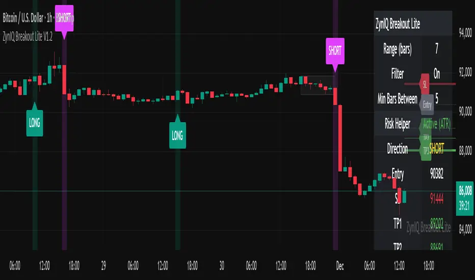
Equal Highs/Lows Multi-Pivot [Julio]Equal Highs/Lows Multi-Pivot
Description
A sophisticated multi-timeframe pivot analysis tool that detects and highlights equal highs and equal lows across four different pivot lengths simultaneously. This indicator identifies price levels where the market creates identical extremes, a powerful signal of institutional support/resistance and potential reversal or breakout zones.
How It Works
Four Independent Pivot Streams
Pivot 1 (Intraday - 2 bars): Ultra-fast level detection for scalpers
Pivot 2 (Session - 4 bars): Short-term swing levels
Pivot 3 (Daily - 6 bars): Medium-term structural levels
Pivot 4 (Weekly - 9 bars): Long-term institutional levels
Equal High (EQH) Detection
Compares consecutive swing highs and draws a line when two highs are nearly identical within a defined threshold. The indicator uses ATR-based confluence to determine "equality," filtering out noise while catching true market structure.
Equal Low (EQL) Detection
Same logic applied to swing lows, identifying support zones where price repeatedly fails to break below previous lows.
Key Features
Four Simultaneous Timeframes: Analyze intraday, session, daily, and weekly structures all on one chart
ATR-Based Confluence Threshold: Automatically adjusts sensitivity based on current volatility (no fake signals)
Color-Coded Levels: Each pivot length has distinct colors for instant visual identification
Highs: Red, Orange, Yellow, Fuchsia
Lows: Green, Blue, Aqua, Purple
Confirmation Mode: Optional setting to wait for full pivot confirmation before marking levels
Customizable Alert Zones: Toggle individual pivot lengths on/off to reduce clutter
Smart Label Positioning: Labels auto-center between the two equal pivots for clarity
Ideal For
Swing traders tracking support/resistance across multiple timeframes
Scalpers identifying micro-structure for quick entries and exits
Market structure analysts studying institutional price action patterns
Multi-timeframe traders needing confluence from intraday to weekly levels
Anyone trading 1-minute to 4-hour charts
Trading Applications
Identify strong support/resistance zones: Equal levels = confirmed institutional levels
Confirm trend reversals: Multiple equal lows = strong accumulation zone; multiple equal highs = distribution
Plan entries with precision: Enter near equal levels for higher probability setups
Detect liquidity concentration: Where price repeatedly tests the same level
Multi-timeframe confluence: Look for equal levels across multiple pivot lengths for ultra-strong zones
How to Use
Identify the equal levels: Color-coded lines instantly show where price creates matching extremes
Check for confluence: Strong setups occur where multiple pivot lengths align
Wait for price action: Watch for breakouts through equal levels or reversals at these zones
Enter with structure: Use equal levels as entry/exit triggers combined with your trading methodology
Manage with confidence: These levels mark institutional decision points
Customization Options
Adjust pivot lengths to match your preferred timeframe structure
Set ATR threshold sensitivity (lower = stricter equality, higher = more signals)
Toggle confirmation mode for additional filter
Enable/disable individual pivot streams to reduce visual clutter
Customize colors to match your chart theme
Default Settings Optimized For
NASDAQ futures and liquid forex pairs
Intraday and swing trading (1-minute to 4-hour charts)
Smart Money / ICT trading methodologies
Volatility-adjusted confluence detection
